2 Spherical Tensegrities

1The three-strut Tensegrity described in Chapter 1 is asymmetrical, having triangular ends and rhomboidal sides. It is the simplest member of an infinitely large family of Tensegrity prisms (T-prisms), analyzed in Appendix 1.1. All of these have rhomboidal sides and none can be made omni-symmetrical. Even the four-strut version (T-4 prism) has plane squares at two ends but twisted squares on four sides.

2 Since we are approaching the design of a dome, we want a Tensegrity whose face patterns, when projected onto a sphere, will divide the sphere’s surface into symmetrically placed zones. The simplest Tensegrity of this kind employs 6 struts arranged in parallel pairs (Diagram 2.1 2.1).

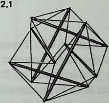
4Again the reader should stop and construct a model. There is nosubstitute for experimenting with an actual structure. Use dowels for the struts as before, and make the tendons 0.6 times their length. (For large models, the theoretical ratio is $1 : 0.6124$ .) When the 24 tendons are in place, it will be found that the parallel strutsare spaced exactly half a strutlength apart, centerline to center-line. We also discover that when two parallel struts are movedtoward or away from each other, the other two pairs move in exact concert. The entire structure expands or contracts symmetrically; it does not bulge here to accommodate a dimple there. The reason the struts will move at all is that the residual elasticity of the tendons is greatly multiplied by the geometry of the system. Elasticity Multiplication—to be examined later—is a characteristic inherent in Tensegrities.

5 This six-strut, twenty-four-tendon Tensegrity has no redundant parts. Each strut is held in place by the cooperative action of a system that comprises twenty-nine other members. When a strut is displaced by application of stress, the whole system undergoes symmetrical modification to accommodate the local movement. The system’s symmetry is not deformed; the system expands as a whole or contracts as a whole. To permit this, each of the eight equilateral triangles rotates about its center; an inward or outward motion of the struts is accompanied by a rotary motion of the tension triangles. Obviously, this ability to respond as a system would be a valuable characteristic of large space-enclosure structures. Ability to respond as a system means that local stresses are being uniformly transmitted throughout the structure, and uniformly absorbed by every part of it. This principle points toward valuable economies in material. Instead of designing every part of the system to receive unassisted whatever loads it may incur, with consequent local accretions of weight and bulk, we may instead design the system on the assumption that local stress will be transmitted throughout its extent, and shared by all its members. The normal state of the system is not a state of rigidity but a state of equilibrium, to which, when disturbed, it seeks to restore itself.

2.1 Equilibrium

6When the tension members of a Tensegrity are taut, it is in a state of equilibrium. To this state, however stressed, it always seeks to return. Unlike the ‘‘straightness’’ of Euclidean lines, the tautness of tension members is an approximation only. The weight of the cord or cable, however slight, will always curve it slightly; turnbuckles and fastenings have always residual slackness; materials have always residual elasticity. It is impossible to pull any line so tight that it could not, with sufficient effort, be pulled a little tighter. Hence the capacity of the system to absorb displacements and restore itself. Still, for purposes of study and of system design, we can imagine an ideal state of equilibrium in which tendons pull perfectly straight and are perfectly tight, and predict the place every component would occupy if the ideal equilibrium could be realized with actual materials.

7 Examination of the six-strut Tensegrity discloses four tendons attached to each strut end. By recourse to a chemical metaphor, we may call it a Valence-4 Tensegrity, it is the simplest of a very large family of these. (The T-prism we examined in Chapter 1 has three tendons per strut end and is hence an example of the Valence-3 Tensegrity family.)

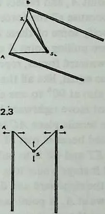
8 The design procedure for a Valence-4 Tensegrity commences from the fact that each strut lies at the bottom of a tensional ‘‘valley’’ whose sides are triangular. Other struts are attached to the apexes of these triangles (Diagram 2.2). Each triangle consists of two tendons plus the strut they share in common. Each pair of tendons, together with the strut, lies in a plane we may call a tensile plane. So each strut lies along the intersection of two tensile planes. (Two intersecting planes, according to projective geometry, suffice to determine the position of a line. This fact may help us understand why the struts tend to stay in place.)

9 We may now examine the conditions of system equilibrium (Diagram 2.3). Since equilibrium is not a static condition of being ‘‘at rest,’’ but rather the resolution of forces that are pulling in several directions, the way to locate it is to examine the forces that are seeking to disrupt it. In the figure, which is Diagram 2.2 redrawn in a different perspective, $S$ is the cross-section of a strut lying at the bottom of a tensile valley ASB. Struts and $B$ are being pulled symmetrically outward, left and right, by other tendons in the system. If they were to obey this pull, they would lift strut $S$ outward and upward. As this happened, angle $𝐴𝑆𝐵$ , the angle between the two tensile planes that locate strut $S$ , would tend to increase.

10 But other tendons attached to strut $S$ are restraining it from moving in this way. They are doing this by pulling it downward and inward. If they were to succeed, strut $S$ , in moving downward, would pull struts $A$ and $B$ inward, and angle $𝐴𝑆𝐵$ , the angle between the two tensile planes that locate strut $S$ ,would tend to decrease.

12 So we can see that the forces in balance are determining angle $𝐴𝑆𝐵$ , the angle between the two tensile planes that locate strut S. Since the system is omni-symmetrical, the pairs of tensile planes associated with each strut will all be at this angle to one another. 2.2 We may call it the dip angle, since the spherical contour of the system here dips inward, incising the polyhedron with a reentrant angle. There is a characteristic dip angle for every symmetrical Valence-4 Tensegrity system. We may intuit, and shall later prove in detail, that if we know the dip angle we can deduce all the system’s component lengths and positions. So our first job is to find the dip angle of the system under consideration.

13 To deduce the dip angle of the six-strut Tensegrity system, we scrutinize the balance of forces more closely (Diagram 2.4). Concentrate on point $A$ , and reflect that in the equilibrium state it stays where it is because all the forces that pull on it are in balance. We may specify some of these forces. The tendons in the tensile plane $𝐴𝑆$ are pulling point $A$ downward and rightward. The rightward and downward forces, represented by the heavy arrows, may be regarded as equal, like all the other sets of forces in the system. They are also at 90° to one another.

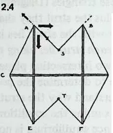
15 Point $A$ does not move rightward because part of the effort of the tendons in the tensile plane $𝐴𝐶$ is to pull it leftward. It does not move downward because part of the effort of the tendons in the tensile planes $𝐸𝑇$ and $𝐶𝐸$ is to pull strut $𝐴𝐸$ upward. These pulls balance, and it stays where it is.

16 Now return to the rightward and downward forces represented by the heavy arrows at $A$ . A point pulled upon by two equal forces will behave as though it responded to a single force, the angle of which is midway between them. So point $A$ responds to a force pulling downward and rightward at 45° to the horizontal and vertical.

17 Similarly, the tensile plane $𝐵𝑆$ pulls the point $B$ downward and leftward at 45°. Being at 45° to the horizontal, the tensile planes and $𝐵𝑆$ are at 90° to each other. The dip angle is the angle between these planes. Thus we have found that in the symmetrical six-strut Tensegrity system the dip angle is 90°.

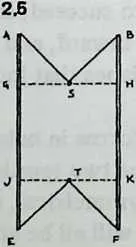
19 We can now proceed more rapidly. Diagram 2.5 shows the same view of the system as Diagram 2.4, but with strut $𝐶𝐷$ omitted and with dotted lines $𝐺𝐻$ and $𝐽𝐾$ drawn through $S$ and $T$ . $𝐺𝐽$ is the separation between struts $S$ and $T$ , and since the system is symmetrical this will be equal to $𝐺𝐻$ , the separation between struts $𝐴𝐸$ and $𝐵𝐹$ . Moreover, since the dip angles $𝐴𝑆𝐵$ and $𝐸𝑇𝐹$ are both 90°, $𝐴𝐺 = 𝐺𝑆$ and $𝐽𝐸 = 𝐽𝑇$ . But we know from symmetry that $S$ is the midpoint of $𝐺𝐻$ , and $T$ is the midpoint of $𝐽𝐾$ . Since we have already found that $𝐺𝐻 = 𝐺𝐽$ , we see that $𝐴𝐺$ and $𝐽𝐸$ must each equal half of $𝐺𝐽$ . Adding $𝐴𝐺, 𝐺𝐽,$ and $𝐽𝐸$ (or $\frac{1}{2} + 1 + \frac{1}{2}$ ), we learn that $𝐺𝐽$ equals half the length of the strut $𝐴𝐸$ . But we know that $𝐺𝐽$ corresponds to the separation between the struts $S$ and T. And all strut separations are alike. So we have shown that in a symmetrical six-strut Tensegrity system the separation between any two parallel struts is exactly half the length of a strut.

20 This fact defines the condition of the system when it is in equilibrium. The struts can only be displaced from half-length separation by a force from outside the system—an inquisitive hand, a falling tree, the pull of gravity on strut materials. Once displaced, half-length separation is the condition to which they will seek to return.

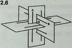
21 It is now a simple matter to calculate tendon lengths for tautness in the equilibrium condition. Diagram 2.6 shows how the pairs of struts are arranged in three mutually perpendicular (orthogonal) planes. In the six-strut Tensegrity system the ends of parallel struts need never be connected; a pair of struts joined by a tendon will always be at a 90° angle to one another. And by symmetry, all twenty-four tendons are of equal length. So there is only one tendon orientation to be considered, and we need only find the length of one tendon.

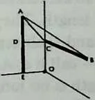
23 Diagram 2.7, a detail extracted from Diagram 2.6, shows the intersection $O$ of the 3 planes, like the meeting of two walls and a floor. Half a strut $𝐴𝐸$ is painted on one wall; the other half is below the floor. Half a strut $𝐶𝐵$ is painted on the adjoining wall; the other half is in the far room. Thus $𝐴𝐸$ and $𝐶𝐵$ equal half a strut length each. $𝐸𝑂$ is half the separation between two parallel struts, thus equals 1/4 strut length. Likewise $𝐶𝑂$ = $1 ∕ 4$ strut length. Thus $𝐴𝐷 = 𝐷𝐶$ . We now have the dimensions we need to solve the right-angled triangle $𝐴𝐷𝐶$ , the hypotenuse of which is a side of the right-angled triangle $𝐴𝐶𝐵$ . The hypotenuse of the latter in turn may be calculated; it is $0.612 4^{+}$ . This is the length of the tendon joining strut ends $A$ and $B$ .

24 Thus for strut length = 1, each of the 24 tendons of a symmetrical 6-strut Tensegrity system is $\sqrt{\frac{3}{8}}$ , or $0.6124$ approximately.

25 We emphasize once more that this is an ideal Tensegrity system with weightless struts and ideally straight tendons. We have calculated design-center values, to which no actual model, large or small, will ever exactly correspond. In a large structure, say with 10-foot struts, the catenary sag of the tendons will always be effective though it may not be readily measurable. Moreover, strut weight will compress the system somewhat; triangles will rotate and tendons will stretch to accommodate this. And whether the model is made large, with beams and cables, or small, with dowels and string, perfect symmetry will prove impossible of attainment, however carefully dimensions are measured. These facts mean only that an actual Tensegrity structure is never quite in the calculated equilibrium state. We recall, however, from experimenting with a model that it has a unique ability to accommodate departures from equilibrium. It can be designed and constructed as though perfect equilibrium were attainable, and will simply accommodate to the deformities introduced by the physical characteristics of materials.

26 So we may want to know what we can predict about the system’s behavior under stress.

2.2 Elasticity Multiplication

27When the system is under stress and hence no longer in equilibrium, the pairs of parallel struts remain parallel but their separation is no longer 1/2 strut length. They have moved either closer together or further apart, and their separation is some new multiple of a strut length—call it $s$ . As the struts move, the tendons stretch. Their length is no longer $0.6124 \times strut length$ , but some greater multiple of a strut length: call it $t$ .

28 To find how $s$ and $t$ are related, we may redraw Diagram 2.7 and label the distances $𝐶𝑂$ and $𝐶𝐷$ not $1 ∕ 4$ but $s ∕ 2$ . (The length of the portions of struts we are dealing with is still $1 ∕ 2$ ; only the strut separation has changed, from $1 ∕ 2$ to $s$ , so the half-separation shown in Diagram 2.8 is no longer $1 ∕ 4$ but $s ∕ 2$ .) The right-angled triangle $𝐴𝐷𝐶$ now has $s ∕ 2$ and $(1 ∕ 2 - s ∕ 2)$ for sides, and $A C^{2}$ becomes $(2 s^{2} - 2 s + 1) ∕ 4$ . Solving triangle $𝐴𝐵𝐶$ with the help of this, we find that $𝐴𝐵$ , the tendon $t$ , is $\sqrt{(s^{2} - s + 1) ∕ 2}$ , when $s$ and $t$ are multiples of strut lengths.

29 We know the value of $t$ when the separation $s$ is $1 ∕ 2$ at the equilibrium condition. Sure enough, if we put $0.5$ for $s$ in this equation, we obtain $t = \sqrt{0.375}$ , or $0.6123724357$ (to ten places).

30 We have obtained a general tendon-length equation for the symmetrical 6-strut Tensegrity:

t = \sqrt{\frac{(s^{2} - s + 1)}{2}} .

(2.1)

31 We are now ready to see what happens if we change the strut separation. Let us try increasing it by 1 percent, a modest increment, well within the stretching capacity of any likely tendon material. We may first define what we might expect to happen.

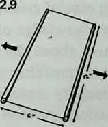
33 Diagram 2.9 shows a pair of parallel struts 12 inches long. They are joined at both ends by strings 6 inches long, so that the strut separation is half a strut length, exactly as with a six-strut Tensegrity in the equilibrium condition. If we now force them apart an additional 1 percent, the separation will have increased from $0.5$ to $0.505$ , a mere $0.06$ inch. The strings will have no difficulty stretching that far, and we are unsurprised to find that the string length has also increased by the same percentage. To write this compactly, we may use the mathematician’s usual symbol, $Δ$ , for the amount of change. The change in strut separation, $Δ s$ , is 0.06 inch; the change in separation expressed as a percentage, $Δ 𝑠%$ , is 1. And the tendon length changes are exactly the same: $Δ t$ is 0.06 inch, $Δ 𝑡%$ is 1. So $Δ s ∕ Δ t = 1$ , and $Δ 𝑠% ∕ Δ 𝑡% = 1$ .

34 To find out what happens when we move two parallel struts of a six-strut Tensegrity apart by the same amount, we have only to solve Equation 2.1, putting 0.505 in place of $s$ . When we do this we find that $t$ , the tendon length, has become $0.6123826418$ . The reader will now see why we calculated the equilibrium tendon length to ten places a page or so back: the difference between the tendon length at equilibrium ( $0.6123724357$ ) and for strut-spacing 1 percent greater than at equilibrium ( $0.6123826418$ ) commences to show up only in the fifth place. The difference is 0.0000102061. In a model with 12-inch struts, separating the struts an additional 1 percent causes the strings to stretch about one ten-thousandth of an inch, which is quite unmeasurable. Dividing separation change by tendon stretch, we obtain not $Δ s ∕ Δ t = 1$ , but $Δ s ∕ Δ t = 489.9$ .

35 The elasticity of tensile materials is usually expressed as a percentage of a unit length. Converting the tendon stretch into a percentage, we find that each tendon has stretched $0.00166$ percent while the strut separation was increasing 1 percent. So $Δ 𝑠% ∕ Δ 𝑡% = 600$ . If we handled the Tensegrity with our eyes shut, imagining that we were holding merely two sticks tied together, as in Diagram 2.9, we should think the tendon material was 600 times more elastic than it actually is. We are encountering the capacity of the system to multiply the elasticity of the tendon material.

36 We have here a classic case of synergy: behavior of whole systems, unpredicted by knowledge of the parts or of any subset of parts. Nothing we know about the struts and strings could allow us to predict their extraordinary behavior when they are united in a six-strut Tensegrity system.

37 It follows that calculations pertaining to such a system, taking into account the known characteristics of the materials but presuming the usual methods of assembling them, are certain to be wrong. We might suppose that if the struts were displaced by 10 percent a tendon would break, because our tendon material will not stretch 10 percent without breaking. But a little work with Equation 2.1 will show that a 10 percent strut displacement (from 0.5 to 0.55) changes tendon length by only 0.00102, a mere 0.167 percent. This is only 1/60 of what we might have expected $(Δ 𝑠% ∕ Δ 𝑡% = 60)$ , and well within the elastic capabilities of any tension material we are likely to think of. By analogy, the tensile network hidden in geodesic domes quite defeats all normal calculations of their strength.

38 The reader will have noticed that when we increased the strut displacement from 1 percent to 10 percent, the ratio of separation change to tendon stretch $(Δ 𝑠% ∕ Δ 𝑡%)$ dropped from 600 to 60. This is generally true of Tensegrity structures: the elasticity multiplication is very great for small displacements (for instance $122, 000$ for a displacement of $0.002$ percent), and drops rapidly as displacement increases (about 10 for displacement of 60 percent). Thus Tensegrities are extremely resilient under light loads. A complex Tensegrity model is never quite still, however tightly the tendons are stretched. On the other hand, it stiffens rapidly as loading increases.

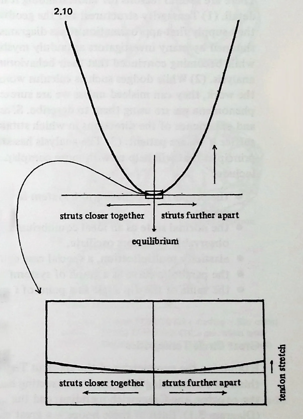
39 We may also wonder what will happen if we push the struts of the 6-strut Tensegrity closer together instead of pulling them apart. The answer is, exactly the same thing. If we decrease the separation by 1 percent, to 0.495, and insert this value into . Equation 2.1, we shall obtain the same tendon stretch as before, and the same $Δ 𝑡% ∕ Δ 𝑡%$ ratio, 600. Whether we expand the system or contract it, the tendons stretch, and at exactly the same rate for the same percentage of change. So the system seeks equilibrium exactly as a ball seeks the bottom of a bowl. A graph of the $s ∕ t$ relationship is in fact bowl-shaped; more precisely, parabola-shaped. Any equation such as Equation 2.1, in which one quantity’s variation is affected by the second power of another, will give us a parabola, if we plot points from it (Diagram 2.10 2.2).

40 The parabola has a theoretical zero point, where it touches the baseline, but this resembles the famous ideal point with position but no magnitude: we can never really say that it is occupied. In the real universe where winds blow, invisible forces tug, and molecules are in ceaseless motion, a Tensegrity will no more quite settle down than will anything else: there will always be minute motions, tiny strut displacements at the order of magnitude where elasticity multiplication is truly enormous and compensating forces have enormous advantage. The parabola’s zero point is that ideal condition of rest which nothing real ever attains, and about which a Tensegrity in particular dances an eternal jig of pre-Socratic derision.