13 Ellipses and Superellipses
1So far we have acquired nothing, except some understanding, that couldn’t be contained in a comprehensive table of chord factors. The real interest of the spherical coordinates, making them worth the labor of computing them, is the way they facilitate geodesicizing nonspherical envelopes. The obvious profile to start with is the ellipse, and the most compact way of tackling the ellipse is to think of it as a member of a large family of shapes with a common mathematical description. We may look at the general equation first, and then move to simple cases by taking things out of it:
2 Here , and are ordinary Cartesian coordinates, at angles to one another; are any positive quantities you like. By varying them we can describe a surprising array of symmetrical shapes: a brick, a modified egg, a sphere, an octahedron (stretched or regular), a pair of crossed lines, a circle, any ellipse at all, not to mention various cigar shapes and squares with rounded corners. We may start in two dimensions by letting , which suppresses the third fraction entirely. Then if and are both 1, and and both 2, we get
3 which describes a circle centered at .
4 The radius of the circle, of course, doesn’t change. To get a changing radius we insert the terms and b. It is easiest to let a = 1 and take up all the variation in b. This gives us
5 which describes an ellipse. We see at once that if = 1 this equation is no different from that of the circle. Obviously determines how the radius varies as we travel round the curve. It is, in fact, the ratio (see Diagram 13.1) of the long and short axes, and to help ourselves remember this we may give it a name, , for expansion.
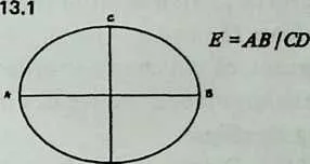
7 So the radius of the ellipse will vary between and 1, and an ellipse with an expansion of, say, 1.5 will be 1.5 times as long as it is broad. If this curve describes the profile of a dome with equatorial truncation, then the dome will have a radius of 1 at ground level and a radius of at the zenith. It is handy to let the floor radius ; then if the dome will be tall for its girth, and if the dome will be flattened. We can thus increase or diminish the headroom without altering the area of the circular floor.
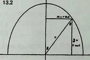
8 To design the dome we need to know exactly how the radius varies. We know that , and from Diagram 13.2 we see that and . Inserting these values for and and rearranging, we obtain our first useful expression:
| (13.1) |
10 In Chapter 9 we calculated a very simple ( octa) dome using Equation 9.1, which gives us chord factors between two points of different radius. was 1.5, and we made a table in which one value had to be taken on trust. (It is now evident how it was arrived at.) For more ambitious cases we proceed in exactly the same way:
- 1.
- from the coordinate table, list the values of 0 that occur between the zenith and the truncation plane;
- 2.
- using Equation 13.1, obtain a value of for each 0; and
- 3.
- use Equation 9.1 to calculate the chord factors, being careful to use the proper pair of for each pair of s.
13.1 Octahedral Ellipsoids
11As usual, the octahedron is the easiest to handle. Its natural equatorial truncation keeps us out of trouble. Sliced at the equator, it yields a beehive shape with a circular floor. By slicing it down the long axis we obtain an elliptical floor, with a semi-elliptical profile as viewed from the side and a semicircular profile as viewed from the end.
12 Such figures, of which one profile is circular, are called ellipsoids of revolution, because we can imagine their being generated by twirling an ellipse.
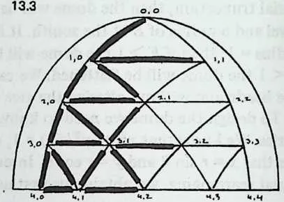
14Example 3Diagram 13.3 shows the coordinate diagram for a octa. For , the 6 values and radii are:
16r | |
170 | 181.5 |
1918.4349488 | 201.4142136 |
2135.2643897 | 221.2602521 |
2345.0 | 241.1766968 |
2565.0051575 | 261.0497813 |
2771.5650512 | 281.0289915 |
2990.0 | 301.0 |
31 Chord factor 0,0/1,0 is obtained with Equation 9.1, using theradii
32 of 0,0 and 1,0 (1.5 and 1.4142136, respectively). It is 0.474423.
33 Fifteen more chord factors are calculated in this way, accounting
34 for every length in the left half of the diagram. Mirror symmetry
35 takes care of the rest.
3637Chord Factors
380,0/1,0 | 390.474423 | 402,1/3,1 | 410.696631 |
421,0/1,1 | 430.632456 | 443,1/3,2 | 450.606092 |
461,0/2,0 | 470.638578 | 483,0/4,0 | 490.326266 |
501,0/2,1 | 510.605791 | 523,0/4,1 | 530.454575 |
542,0/2,1 | 550.635872 | 564,0/4,1 | 570.320364 |
582,0/3,0 | 590.526758 | 603,1/4,1 | 610.452409 |
622,0/3,1 | 630.589150 | 644,1/4,2 | 650.459506 |
663,0/3,1 | 670.456607 | 683,1/4,2 | 690.532697 |
70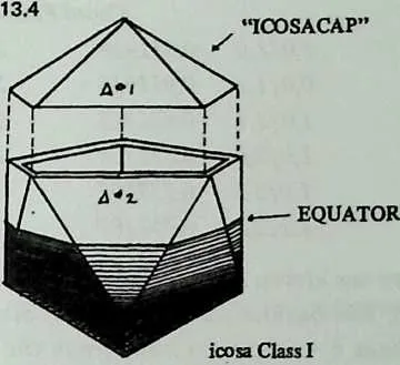 Icosahedral Ellipsoids
71The five-way symmetries of the icosahedron make for especially
72beautiful ellipsoidal patterns. This important advantage is its
73principal one. As soon as we depart from spherical profiles, we
74lose a virtue we have come to expect of the icosa, a relatively small
75inventory of different strut lengths. Unless we are going to settle
76for ridiculously shallow truncations, we must cope with two
77different face triangles. This is clear from Diagram 13.4, where we
78see the icosa dissected into (1) Fuller’s ‘‘icosacap,’’ the set of five
79triangles surrounding the zenith, and (2) the set of ten triangles
80around the waist. It is clear that we must enter this second set to
81find the equator, and that the two sets will be stretched or
82squashed in different proportions as the radius swings down. So
83the icosa Class I tables provide coordinates for a second triangle.
84In the same way, the icosa Class II tables cover five Class II tri-
85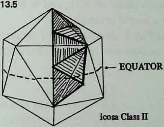 angles: Diagram 13.5 shows how they are located on the icosa.
86We shall work an example from each class, and to keep the work brief we shall stick to 2v.
87Example 42v icosa Class II. Diagram 13.6 shows the vertex diagram for the five Class II triangles. The coordinates are quickly listed from the table, and the radii calculated:
880 | 90r | ||
910,1 | 920 | 930 | 947.5 |
951,0 | 960 | 9737.3773681 | 981.2411302 |
991,1 | 10072 | 10137.3773681 | 1021.2411302 |
1032,0 | 1040 | 10579.1876830 | 1061.0099209 |
1072,1 | 10836 | 10963.4349488 | 1101.0606601 |
1113,0 | 1120 | 113116.5650512 | 1141.0606601 |
1153,1 | 11636 | 117100.8123170 | 1181.0099209 |
119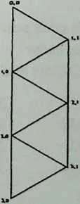 The symmetries above and below the line
are evident from the
12013.6
121 table of radii above: 2,0 corresponds with 3,1 and 2,1 with 3,0. To
122 see how this works out in distances, we shall this time list all the
123 chord factors:
124125Chord Factors
1260,0/1,0 | 1270.911918 | 1282,0/2,1 | 1290.665207 |
1300,0/1,1 | 1310.911918 | 1322,1/3,1 | 1330.665207 |
1341,0/1,1 | 1350.885725 | 1362,0/3,1 | 1370.720724 |
1381.0/2,0 | 1390.831758 | 1402,0/3,0 | 1410.665207 |
1421,0/2,1 | 1430.757107 | 1443,0/3,1 | 1450.665207 |
1461,1/2,1 | 1470.757107 | ||
148 There are eleven distances in the diagram, but only six different ones. The builder would need only six different members.
149 Since occurs nowhere in the coordinate table, no point on this structure lies on an equator. Indeed, we may wonder how we should go about truncating it. Chapter 14 will tell.
150We move on to the second icosa example, a Class I ellipse. This time we shall use a fractional expansion, , to get a saucer rather than a beehive. We shall have fault to find with the first version we come up with, and in learning how to modify it will master a useful principle.
151Example 52v icosa Class I, squashed. The coordinate layout is shown in Diagram 13.7. The figures look like this:
1520 | 1530 | 154r(E = 1/1.5) | |
1550,0 | 1560 | 1570 | 1580.66666667 |
1591,0 | 1600 | 16131.7174743 | 1620.72461704 |
1631,1 | 16472 | 16531.7174743 | 1660.72461704 |
1672,0 | 1680 | 16963.4349488 | 1700.89442719 |
1712,1 | 17236 | 17358.2825255 | 1740.86210372 |
1753,1 | 17618 | 17790.0 | 1781.0 |
1793/2 | 18054 | 18190.0 | 1821.0 |
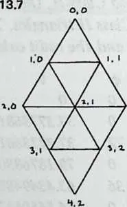
184 Though the coordinate table goes past and , we don’t need any values beyond (the equator). We now compute chord factors and get the following:
185 0,0/1,0
186 1,0/1,1
187 1,0/2,0
188 1.0/2,1
189 0.384256
190 0.447838
191 0.471622
192 0.507459
193 2,0/2,1
194 2,0/3,1
195 2,1/3,1
196 3,1/3,2
197 0.481007
198 0.527551
199 0.590178
200 0.618034
13.2 Modifying Coordinates
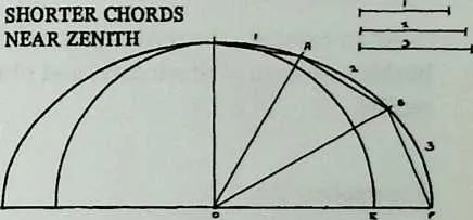
201Study of the chord factors we have just calculated, or better still study of a simple model, will disclose an unwelcome asymmetry: the short members are bunched around the zenith, where they have little to contribute but weight, and the longest members, straddling the most widely separated vertices, are found around the sides where the load is being transmitted to earth. A glance at Diagram 13.8 shows what has happened. Our coordinate system was designed to give reasonably uniform member lengths on a sphere. When a shallow curve intercepts the bundle of sight lines, different struts are differently affected. This is true of course with any non-circular contour, but it is more likely to be troublesome with a shallow ellipse. A beehive may often concentrate its elongations near the zenith with neither aesthetic nor structural harm, since the zenith members have little load to bear.
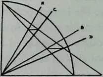
203 Our recourse is to modify the coordinates before doing anything else. Instead of projecting the array against an expanded envelope, we might in effect allow the expansion of the envelope to pull the zenith coordinates apart. This is like reflecting the array off a slanted mirror whose slope is governed by the expansion (Diagram 13.9). Each is replaced by , obtained from
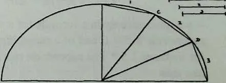
205 Diagram 13.10 shows a typical result. The stretching of chords now tends to parallel the long axis of the ellipse—the reverse of the situation in Diagram 13.8--- and the zenith of a shallow structure is no longer congested with short members. Calculation would also show that the overall variation in strut length is reduced. This procedure gives chord factors identical with those of the elliptical structures in Domebook 2. We may nickname it the E Correction.
206 But there is a simple way to do still better. Replace each by , obtained from
| (13.2) |
207 We may call this the Root E Correction. It distributes the strut lengths very much as the parent sphere did, the longest members part-way down, shorter ones toward zenith and base. And the overall variation of strut lengths is held within close bounds—probably the closest we can easily obtain. In fact the Root E Correction may be recommended as a routine procedure for all elliptical geodesics. For the case we have been discussing it gives these chord factors:
2080,0/1,0 | 209.456149 | 2102,0/2,1 | 211.515500 |
2121,0/1,1 | 213.529609 | 2142,0/3,1 | 215.475770 |
216lj0/2,0 | 217.472080 | 2182,113,1 | 219.530104 |
2201,0/2,1 | 221.542841 | 2223,1/3,2 | 223.618034 |
224 As an exercise, the reader may refigure the Class II icosa beehive we figured previously, and observe the improvement that results.
13.3 Superspheroids
225At the beginning of this chapter we displayed a general equation from which we obtained the equation of the circle by assigning appropriate values. To the two exponents and we assigned the value 2, and we kept 2 for an exponent when we went on to the ellipse. But there is no reason any exponent needs to be 2. It can be anything from zero to infinity. If it is zero, the ellipse or circle equation yields not a curve but a pair of crossed lines. If it is infinity, we obtain a rectangle (or, if , a square). Some years ago the Danish polymath Piet Hein proposed mediating between the circle and the square by making the exponent 2.5. If we modify Equation 13.1 in this way, remembering to insert a 2.5 root as well as 2.5 powers—
| (13.3) |
226 —we have once again a formula for a varying radius, that of a
227supercircle if , and of a superellipse if has some other value, for instance 1.5.1 The supercircle radius formula by itself looks like this:
| (13.4) |
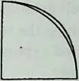
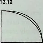
229 A supercircle (Diagram 13.11) is beginning to develop shoulders. A superellipse (Diagram 13.12) has less taper than a normal ellipse of the same expansion. A dome with either profile retains more of its headroom further from the center than does the non-super version. The versatile Peter Calthorpe designed a superspherical icosa some years ago. The one effort I know of to build one encountered legal and financial troubles unrelated to the design.
231 The simplest way to use these shapes is to combine them with a circular floor plan as we did the ellipse. We thus obtain the shape generated by twirling a supercircle or a superellipse on its axis: a superspheroid or a superellipsoid of revolution.
232 The (or y*) function on the calculator makes 2.5 almost as easy an exponent to use as 2. (We get the 2.5th root by raising to the power ). Radius tables and then chord factors are obtained exactly as they were earlier in this chapter. The reader should have no difficulty obtaining the following chord factors for a octa supersphere:
2330,0/1,0 | 2340.326072 | 2353,0/3,1 | 2360.454425 |
2371,0/1,1 | 2380.459825 | 2393,0/4,0 | 2400.326072 |
2411,0/2,0 | 2420.484335 | 2433,014,1 | 2440.454351 |
2451,0/2,1 | 2460.460526 | 2473,1 /4.1 | 2480.449895 |
2492,0/2,1 | 2500.552911 | 2514,014,1 | 2520.320364 |
2532,0/3,0 | 2540.484335 | 2554,114,2 | 2560.459506 |
2572,0/3,1 | 2580.547799 | 2593,114,2 | 2600.529997 |
2612,1/3,1 | 2620.608369 | 2633,1 /3,2 | 2640.601483 |
265 Two of these are duplicated, so the octa supersphere requires 14 different components, as against 6 for a normal sphere. Careful study of a model is the only way to decide if it is worth the complication.
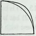
266 Just as 2 is an optional exponent, so is 2.5. The latter has no special magic except that
Piet Hein likes the curves it generates. By raising the supersphere exponent to 3, we
can retain headroom even further from the center, But another way of putting this
is
that we are making a large area around the zenith nearly flat (see Diagram 13.13). The spherical
excess of the structure is concentrated in a rather narrow zone where roof suddenly becomes wall.
Nearly flat areas in geodesic structures are areas of potential trouble, requiring careful hub
detailing to retain the integrity of the tension network. Stretching the supercircle into a
superellipse expands the problem area, and exponents above 2.5 are not recommended for
superellipses.
13.4 Varying Two Radii
268The sphere is a circle of revolution; the supersphere is a supercircle of revolution; the ellipsoids we have considered have been ellipsoids of revolution. This simply means that one cross-section is circular, and such domes, unless they are truncated obliquely, will have either a circular floor plan and a special profile, or a special floor plan and one semicircular profile. The structure’s native sphericity is expanded (or contracted) in only one direction.
269 But there is no reason why we cannot vary two radii. This means specifying two separate expansions, and , one for the floor and the other for the profile. (Separate need not mean different both expansions may have the same value, but they will both make their presences felt.) So we could have a supercircular profile, to get headroom, and a superelliptical floor plan, to get walking space. The respective expansions would be 1 and something else, say 1.25. The exponents could be the same, or different. The structure would have no circular cross-section at all.
270 Since the radius of each vertex is now responding to two expansions, and perhaps to two exponents, the arithmetic becomes more labyrinthine. Still, all we need to calculate chord factors is a table of radii as measured from a central point, and we can make one if we keep our heads.
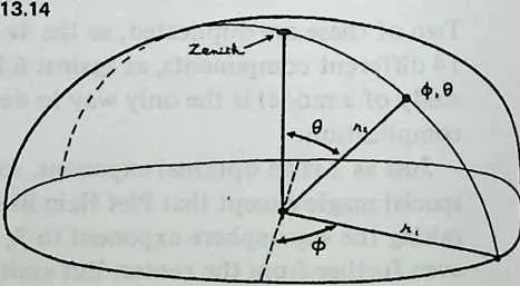
272 Diagram 13.14 shows the situation. We want the radius from the center of the system to vertex . We first assume a floor plane passing through the center (though when we are finished nothing will prevent us putting the floor somewhere else). We next want which is the radius of the floor at the point where the meridian through the vertex in question crosses its edge. This radius is a function of , the expansion of the floor ellipse, and of the of the vertex in question. Its equation is:
| (13.5) |
273 We might tabulate for every pertinent value of 0, which means for one-quarter of the dome’s perimeter, and use it to obtain r2, the radius we want for chord factors, as follows:
| (13.6) |
274 But we should go to all this trouble only in the unlikely case when we might want to use different values of the exponent for the two radii. The exponent is, of course, 2 for ellipses and normally 2.5 for super circles and superellipses, and it seems ill-advised to mix the two in one structure. So we take advantage of the fact that when the two exponents are identical the two equations collapse into one:
| (13.7) |
275 (The exponent , if you’ve forgotten, means the th root.)
276 For high jinks of this kind the octahedron has obvious advantages, since one face triangle takes care of the whole quadrant and brings us clear down to the equatorial truncation line. In Chapter 15 we shall look at its disadvantages, which stem from the way its tendency toward flatness at the square vertices is accentuated by the flat areas peculiar to the superellipse.
277 The icosa remains elegant and far from impossible. In Chapter 15 we shall develop a fancy application in detail, and a worked example is deferred until then.
278 A few pages back we found that it was sometimes desirable to improve the symmetry of a non-spherical form by modifying one coordinate; Equation 13.2 gave a convenient method. Now that we are dealing with two expansions the symmetry has more ways of becoming displeasing, and improving it will mean modifying both coordinates. An elegant result is obtained by changing 0 to 0p:
| (13.8) |
279 and to .
| (13.9) |
280 These expressions reproduce the effect of projecting points onto a sphere and then expanding it, rather than projecting spherical coordinates onto an already expanded envelope. The designer will have to judge whether they are worth the bother.
281 They assume, too, that the floor is being expanded along the axis, an innocuous assumption if we are using the octahedron, whose and axes are indistinguishable. Chapter 15 shows that with the icosahedron there is reason to make a decision, and should we decide to expand its floor along the axis, we need to alter both equations slightly. In Equation 13.8 the division becomes a multiplication, and in Equation 13.9 ‘‘’’ and ‘‘’’ must be interchanged.
13.5 Free Forms
282It is possible to apply the geodesic three-way grid to any surface that can be mathematically described. The description is not always easy, and one can conceive of convex curves that would give a skilled mathematician trouble. One thing that is simple in spherical coordinates, though, is the notation for any surface of revolution whose profile is a convex curve drawn freehand. Should you want a shape like the one in Diagram 13.15, you have only to draw it on graph paper, designate an origin point, and from that point run radii out to the curve, the angle of each radius with the vertical axis being one of the values for the breakdown you have chosen. Call the length of the vertical axis , and measure the other radii. Then use those radii, and the values from the table for your breakdown, in Equation 9.1 to get chord factors. The octahedron’s seams make it possible to combine two such profiles, left and right. Keep the roofline convex and avoid extended arcs of very low curvature, unless you are prepared to take the structural measures described in Chapter 16.