::: center
Regular Polytopes
:::
::: titlepage
Regular Polytopes
H. S. M. Coxeter
Dover Publications | San Antonio
ISBN: 978-0486614809
ISBN-10: 0486614808
Updated: 2024-11-23
:::
::: flushleft
Copyright
All rights reserved. No part of this book may be reproduced or transmitted in any form or by any means, electronic or mechanical, including photocopying, recording, or by any information storage and retrieval system, without permission in writing from the Copyright Holder.
ENCODED IN THE UNITED STATES OF AMERICA
:::

¶ Table of Contents
[PREFACE TO THE THIRD EDITION]{.underline}
[PREFACE TO THE FIRST EDITION]{.underline}
[Table of Contents]{.underline}
[Table of Figures]{.underline}
[CHAPTER I - POLYGONS AND POLYHEDRA]{.underline}
[CHAPTER II - REGULAR AND QUASI-REGULAR SOLIDS]{.underline}
[CHAPTER III - ROTATION GROUPS]{.underline}
[CHAPTER IV - TESSELLATIONS AND HONEYCOMBS]{.underline}
[CHAPTER V - THE KALEIDOSCOPE]{.underline}
[CHAPTER VI - STAR-POLYHEDRA]{.underline}
[CHAPTER VII - ORDINARY POLYTOPES IN HIGHER SPACE]{.underline}
[CHAPTER VIII - TRUNCATION]{.underline}
[CHAPTER IX - POINCARÉ’S PROOF OF EULER’S FORMULA]{.underline}
[CHAPTER X - FORMS, VECTORS, AND COORDINATES]{.underline}
[CHAPTER XI - THE GENERALIZED KALEIDOSCOPE]{.underline}
[CHAPTER XII - THE GENERALIZED PETRIE POLYGON]{.underline}
[CHAPTER XIII - SECTIONS AND PROJECTIONS]{.underline}
[CHAPTER XIV - STAR-POLYTOPES]{.underline}
[DEFINITIONS OF SYMBOLS USED IN THE FOLLOWING TABLES]{.underline}
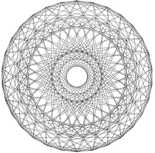
The four-dimensional polytope {3, 3, 5}, drawn by van Oss (cf. Fig. 13.6B on page 250).
[]
[]
To
MY WIFE
[]
Copyright © 1973 by Dover Publications, Inc.
Copyright © 1963 by H. S. M. Coxeter.
All rights reserved.
This Dover edition, first published in 1973, is an unabridged and corrected republication of the second edition published by The Macmillan Company in 1963. It contains a new preface by the author.
Library of Congress Catalog Card Number: 73-84364 International Standard Book Number
9780486141589
Manufactured in the United States by Courier Corporation
61480811
www.doverpublications.com
[]
¶ PREFACE TO THE THIRD EDITION
THIS EDITION follows the second quite closely but embodies more than twenty small improvements. It has not seemed worthwhile to replace the term “congruent transformation” by its modern equivalent “isometry”. Although the first edition appeared as long ago as 1948, the subject remains alive, as can be seen in the success of L. Fejes Tóth’s Regular Figures (Pergamon, 1964), B. Grünbaum’s Convex Polytopes (Interscience, 1967), and M. J. Wenninger’s Polyhedron Models (Cambridge University Press, 1970).
The works of L. Schläfli have been published in three volumes (Gesammelte Mathematische Abhandhungen, Birkhäuser, Basel, 1950, 1953, 1956). Our references “Schläfli 1,2,3,4” (see page 312) can be found there in vol. II, pp. 164-190, 198-218, 219-270, and vol. I, pp. 167-392.
It is, perhaps, worthwhile to mention that the electron microscope has revealed icosahedral symmetry in the shape of many virus macromolecules. For instance, the virus that causes measles looks much like the icosahedron itself. The Preface to the First Edition refers to a passage on page 13 concerning the impossibility of any inorganic occurrence of this polyhedron. That statement must now he taken with a grain of borax, for the element boron forms a molecule B12 whose twelve atoms are arranged like the vertices of an icosahedron.1
The first preface also refers to a missing “fifteenth chapter” on hyperbolic honeycombs. This now occurs as Chapter 10 in my Twelve Geometric Essays (Coxeter 19).
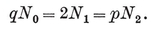
(j,k) = ƒ(j) g(k) − ƒ(k) g(j) ,
where ƒ and g are arbitrary functions. For some interesting consequences, see Chapter 5 of my Regular Complex Polytopes (Coxeter 21).
UNIVERSITY OF TORONTO
H. S. M. COXETER
May 1973
[]
¶ PREFACE TO THE FIRST EDITION
A POLYTOPE is a geometrical figure bounded by portions of lines, planes, or hyperplanes ; e.g., in two dimensions it is a polygon, in three a polyhedron. The word polytope seems to have been coined by Hoppe in 1882, and introduced into English by Mrs. Stott about twenty years later. But the concept, under the name polyscheme, goes back to Schläfli, who completed his great monograph in 1852.
The foundations for our subject were laid by the Greeks over two thousand years ago. In fact, this book might have been subtitled “A sequel to Euclid’s Elements”. But all the more elaborate developments (roughly, from Chapter V on) are less than a century old. This revival of interest was partly due to the discovery that many polyhedra (including three of the regular ones) occur in nature as crystals. However, there is a law of symmetry (4•32) which prohibits the inanimate occurrence of any pentagonal figure, such as the regular dodecahedron. Thus the chief reason for studying regular polyhedra is still the same as in the time of the Pythagoreans, namely, that their symmetrical shapes appeal to one’s artistic sense. (To be sure, there is a little more to it than that : Klein’s Lectures on the Icosahedron2 cast fresh light on the general quintic equation. But if Klein had not been an artist he might have expressed his results in purely algebraic terms.)
As for the analogous figures in four or more dimensions, we can never fully comprehend them by direct observation. In attempting to do so, however, we seem to peep through a chink in the wall of our physical limitations, into a new world of dazzling beauty. Such an escape from the turbulence of ordinary life will perhaps help to keep us sane. On the other hand, a reader whose standpoint is more severely practical may take comfort in Lobat-schewsky’s assertion that “there is no branch of mathematics, however abstract, which may not some day be applied to phenomena of the real world.”
I have tried to make this book as nearly self-contained as is reasonably possible. Anyone familiar with elementary algebra, geometry, and trigonometry will be able to appreciate it, and may find in it some fresh applications of those subjects ; e.g., Chapter III provides an introduction to the theory of Groups. All the geometry of the first six chapters is ordinary solid geometry ; but the topics treated have been carefully selected as forming a useful background for the subsequent developments. If the reader is at all distressed by the multi-dimensional character of the rest of the book, he will do well to consult Manning’s Geometry of four dimensions or Sommerville’s Geometry of n dimensions (i.e., Manning 1 or Sommerville 3).
It will be seen that most of our chapters end with historical summaries, showing which parts of the subject are already known. The history of polytope-theory provides an instance of the essential unity of our western civilization, and the consequent absurdity of international strife. The Bibliography lists the names of thirty German mathematicians, twenty-seven British, twelve American, eleven French, seven Dutch, eight Swiss, four Italian, two Austrian, two Hungarian, two Polish, two Russian, one Norwegian, one Danish, and one Belgian. (In proportion to population the Swiss have contributed more than any other nation.)
This book grew out of an essay on “ Dimensional Analogy ”, begun in February 1923. It is thus the fulfilment of 24 years’ work, which included the rediscovery of Schläfli’s regular polytopes (Chapters VII and VIII), Hess’s star-polytopes (Chapter XIV) and Gosset’s semi-regular polytopes (§§ 8·4 and 11·8). Probably my own best contribution is the invention of the “ graphical ” notation (§ 5·6), which facilitates the enumeration of groups generated by reflections (§ 11·5), of the polytopes derived from these groups by Wythoff’s construction (§ 11·6), of the elements of any such polytope (§11·8), and of “ Goursat’s tetrahedra ” (§14·8). This last instance, which looks like some bizarre notation for the Music of the Spheres, is essentially a device for computing the volumes of certain spherical tetrahedra without having recourse to the calculus. The same notation can be applied very effectively to the theory of regular honeycombs in hyperbolic space (see Schlegel 1, pp. 360, 444, or Sommerville 3, Chapter X), but I have resisted the temptation to add a fifteenth chapter on that subject.
In some places, such as §§ 8·2-8·5, I have chosen to employ synthetic methods where the use of coordinates might have made the work a little easier. On the other hand, I have not hesitated to use coordinates in Chapter XI, where they greatly simplify the discussion, and in Chapter XII, where they seem to be quite indispensable.
Many of the technical terms may be new to the reader, who will be apt to forget what they mean. For this reason the Index (pages 315-321) refers to definitions by means of page-numbers in boldface type. Every reader will find some parts of the book more palatable than others, but different readers will prefer different parts : one man’s meat is another man’s poison. Chapter XI is likely to be found harder than the subsequent chapters.
I offer most cordial thanks to Thorold Gosset, Leopold Infeld and G. de B. Robinson for reading the whole manuscript and making many valuable suggestions. I am grateful also to Richard Brauer, J. J. Burckhardt, J. D. H. Donnay, J. C. P. Miller, E. H. Neville and Hermann Weyl for criticizing various portions, to Mrs. E. L. Voynich for biographical material about her sister, Mrs. Stott (§ 13•9), to Dorman Luke for the gift of his models of polyhedra (which aided me in drawing some of the figures, e.g. in § 6•4), to P. S. Donchian for the eight Plates, to H. G. Forder and Alan Robson for help in reading the proofs, and to Messrs. T. & A. Constable of Edinburgh for their expert printing of difficult material.
H. S. M. COXETER
UNIVERSITY OF TORONTO
April 1947
[]
¶ Table of Contents
Title Page
Dedication
Copyright Page
PREFACE TO THE THIRD EDITION
PREFACE TO THE FIRST EDITION
Table of Figures
CHAPTER I - POLYGONS AND POLYHEDRA
CHAPTER II - REGULAR AND QUASI-REGULAR SOLIDS
CHAPTER III - ROTATION GROUPS
CHAPTER IV - TESSELLATIONS AND HONEYCOMBS
CHAPTER V - THE KALEIDOSCOPE
CHAPTER VI - STAR-POLYHEDRA
CHAPTER VII - ORDINARY POLYTOPES IN HIGHER SPACE
CHAPTER VIII - TRUNCATION
CHAPTER IX - POINCARÉ’S PROOF OF EULER’S FORMULA
CHAPTER X - FORMS, VECTORS, AND COORDINATES
CHAPTER XI - THE GENERALIZED KALEIDOSCOPE
CHAPTER XII - THE GENERALIZED PETRIE POLYGON
CHAPTER XIII - SECTIONS AND PROJECTIONS
CHAPTER XIV - STAR-POLYTOPES
EPILOGUE
DEFINITIONS OF SYMBOLS USED IN THE FOLLOWING TABLES
BIBLIOGRAPHY
INDEX
[]
¶ Table of Figures
Fig. 13.6B
FIG. 1.1A
FIG. 1.4A
FIG. 1.5A
FIG. 1.5B
FIG. 1.6A
FIG. 2.3A
FIG. 2.3B
FIG. 2.4A
FIG. 2.4B
FIG. 2.6A
FIG. 2.8A
FIG. 3.1A
FIG. 3.1B
FIG. 3.4A
FIG. 3.6A
FIG. 3.6B
FIG. 3.6C
FIG. 3.6D
FIG. 3.6E
FIG. 3.8A
FIG. 4.1A
FIG. 4.2A
FIG. 4.2B
FIG. 4.2C
FIG. 4.2D
FIG. 4.2E
FIG. 4.2F
FIG. 4.2G
FIG. 4.3A
FIG. 4.5A
FIG. 4.5B
FIG. 4.7A
FIG. 5.1A
FIG. 5.1B
FIG. 5.1C
FIG. 5.2A
FIG. 5.4A
FIG. 5.4B
FIG. 5.9A
FIG. 5.9B
FIG. 6.1A
FIG. 6.2A
FIG. 6.2B
FIG. 6.2C
FIG. 6.2D
FIG. 6.4A
FIG. 6.4B
FIG. 6.4C
FIG. 6.4D
FIG. 6.6A
FIG. 6.6B
FIG. 6.7A
FIG. 6.7B
FIG. 6.8A
FIG. 6.9A
FIG. 7.2A
FIG. 7.2B
FIG. 7.2C
FIG. 7.9A
FIG. 8.1A
FIG. 8.2A
FIG. 8.2B
**FIG. 8.4A
** **FIG. 8.4B
** FIG. 8.9A
FIG. 10.4A
FIG. 10.8A
FIG. 11.9A
FIG. 12.4A
FIG. 12.4B
FIG. 12.7A
FIG.12.7B
FIG. 13.1A
FIG. 13.2A
FIG. 13.3A
FIG. 13.5A
FIG. 13.5B
FIG. 13.6A
FIG. 13.6B
Fig. 13.8A
Fig. 13.8B
FIG. 14.2A
FIG. 14.3A
FIG. 14.3B
FIG. 14.3C
FIG. 14.8A
The length and the breadth and the height of it are equal.
Revelation 21. 16
That ye, being rooted and grounded in love, May be able to comprehend with all saints what is the breadth, and length, and depth, and height.
Ephesians 3. 17, 18
[]
¶ CHAPTER I
POLYGONS AND POLYHEDRA
TWO-DIMENSIONAL polytopes are merely polygons ; these are treated in § 1·1. Three-dimensional polytopes are polyhedra ; these are defined in § 1·2 and developed throughout the first six chapters. § 1·3 contains a version of Euclid’s proof that there cannot be more than five regular solids, and a simple construction to show that each of the five actually exists. The rest of Chapter I is mainly topological : a regular polyhedron is regarded as a map, and later as a configuration. In § 1·5 we take an excursion into “ recreational ” mathematics, as a preparation for the notion of a tree of edges in von Staudt’s elegant proof of Euler’s Formula.
1·1. Regular polygons. Everyone is acquainted with some of the regular polygons : the equilateral triangle which Euclid constructs in his first proposition, the square which confronts us all over the civilized world, the pentagon which can be obtained by making a simple knot in a strip of paper and pressing it carefully flat,3 the hexagon of the snowflake, and so on. The pentagon and the enneagon have been used as bases for the plans of two American buildings : the Pentagon Building near Washington, and the Bahá’í Temple near Chicago. Dodecagonal coins have been made in England and Canada.
To be precise, we define a p-gon as a circuit of p line-segments A1 A2, A2 A3, . . . , A*p* A1, joining consecutive pairs of p points A1, A2, . . . , Ap. The segments and points are called sides and vertices. Until we come to Chapter VI we shall insist that the sides do not cross one another. If the vertices are all coplanar we speak of a plane polygon, otherwise a skew polygon.
A plane polygon decomposes its plane into two regions, one of which, called the interior, is finite. We shall often find it convenient to regard the p-gon as consisting of its interior as well as its sides and vertices. We can then re-define it as a simply-connected region bounded by p distinct segments. (“ Simply-connected ” means that every simple closed curve drawn in the region can be shrunk to a point without leaving the region, i.e., that there are no holes.)
The most important case is when none of the bounding lines (or “ sides produced ”) penetrate the region. We then have a convex p-gon, which may be described (in terms of Cartesian coordinates) by a system of p linear inequalities

These inequalities must be consistent but not redundant, and must provide the range for a finite integral

(which measures the area).
A polygon is said to be equilateral if its sides are all equal, equiangular if its angles are all equal. If p > 3, a p-gon can be equilateral without being equiangular, or vice versa ; e.g., a rhomb is equilateral, and a rectangle is equiangular. A plane p-gon is said to be regular if it is both equilateral and equiangular. It is then denoted by {p} ; thus {3} is an equilateral triangle, {4} is a square, {5} is a regular pentagon, and so on.
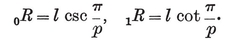
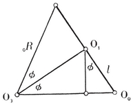
A regular polygon is easily seen to have a centre, from which all the vertices are at the same distance 0R, while all the sides are at the same distance 1R. This means that there are two concentric circles, the circum-circle and in-circle, which pass through the vertices and touch the sides, respectively.
It is sometimes helpful to think of the sides of a p-gon as representing p vectors whose sum is zero. They may then be compared with p segments issuing from one point, the angle between two consecutive segments being equal to an exterior angle of the p-gon. It follows that the sum of the exterior angles of a plane polygon is a complete turn, or 2π. Hence each exterior angle of {p} is 2π/p, and the interior angle is the supplement,
1·11

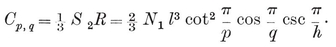
This may alternatively be seen from the right-angled triangle O2 O1 O0 of Fig. 1.1A, where O2 is the centre, O1 is the mid-point of a side, and O0 is one end of that side. The right angle occurs at O1, and the angle at O2 is evidently π/p. If 2l is the length of the side, we have
O**0** O**1** = l, O**0** O**2** = 0R, O1 O**2** = **1**R ;
therefore
1·12
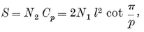
The area of {p}, being made up of 2p such triangles, is
1·13
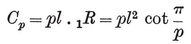
(in terms of the half-side l). The perimeter is, of course,
1·14

As p increases without limit, the ratios S/0R and S/1R both tend to 2π, as we would expect. (This is how Archimedes estimated π, taking p=96.)
We may take the Cartesian coordinates of the vertices to be
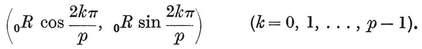
Then, in the Argand diagram, the vertices of a {p} of circum-radius 0R=1 represent the complex numbers e2kπi/p, which are the roots of the cyclotomic equation
1·15

It is sometimes desirable to extend our definition of a p-gon by allowing the sides to be curved ; e.g., we shall have occasion to consider spherical polygons, whose sides are arcs of great circles on a sphere. This extension makes it possible to have p=2 : a digon has two vertices, joined by two distinct (curved) sides.
1·2. Polyhedra. A polyhedron may be defined as a finite, connected set of plane polygons, such that every side of each polygon belongs also to just one other polygon, with the proviso that the polygons surrounding each vertex form a single circuit (to exclude anomalies such as two pyramids with a common apex). The polygons are called faces, and their sides edges. Until Chapter VI we insist that the faces do not cross one another. Thus the polyhedron forms a single closed surface, and decomposes space into two regions, one of which, called the interior, is finite. We shall often find it convenient to regard the polyhedron as consisting of its interior as well as its N2 faces, N1 edges, and N0 vertices.
The most important case is when none of the bounding planes penetrate the interior. We then have a convex polyhedron, which may be described (in terms of Cartesian coordinates) by a system of inequalities

These inequalities must be consistent but not redundant, and must provide the range for a finite integral
(which measures the volume).
Certain polyhedra are almost as familiar as the polygons that bound them. We all know how a point and a p-gon can be joined by p triangles to form a pyramid, and how two equal p-gons can be joined by p rectangles to form a right prism. After turning one of the two p-gons in its own plane so as to make its vertices (and sides) correspond to the sides (and vertices) of the other, we can just as easily join them by 2p triangles to form an antiprism, whose 2p lateral edges make a kind of zigzag.
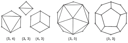
A tetrahedron is a pyramid based on a triangle. Its faces consist of four triangles, any one of which may be regarded as the base. If all four are equilateral, we have a regular tetrahedron. This is the simplest of the five Platonic solids. The others are the octahedron, cube, icosahedron, and (pentagonal) dodecahedron. (See Plate I, Figs. 1-5.)
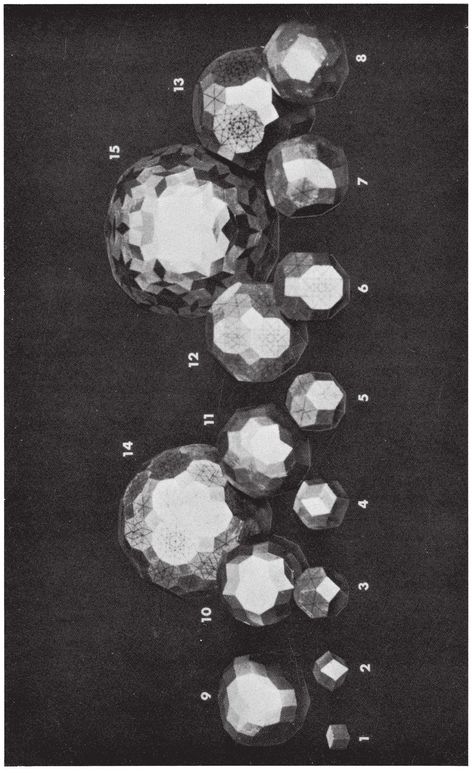
PLATE I
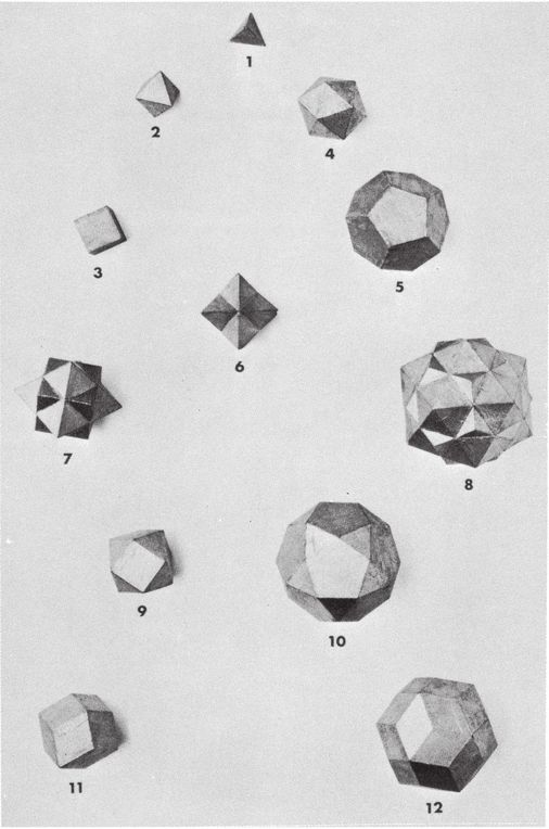
REGULAR, QUASI-REGULAR AND RHOMBIC SOLIDS
1·3. The five Platonic solids. A convex polyhedron is said to be regular if its faces are regular and equal, while its vertices are all surrounded alike. (We shall see in § 1•7 that the regularity of faces may be waived without causing anything worse than a simple distortion. A more “economical” definition will be given in § 2·1.) If its faces are {p}’s, q surrounding each vertex, the polyhedron is denoted by {p, q}.
The possible values for p and q may be enumerated as follows. The solid angle at a vertex has q face-angles, each (1–2/p)π, by 1•11. A familiar theorem states that these q angles must total less than 2π. Hence 1–2/p<2/q ; i.e.,
1·31

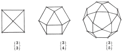
or (p–2)(q–2)<4. Thus {p, q} cannot have any other values than
{3,3}, {3, 4}, {4,3}, {3,5}, {5,3}.
The tetrahedron {3, 3} has already been mentioned. To show that the remaining four possibilities actually occur, we construct the rest of the Platonic solids, as follows.
By placing two equal pyramids base to base, we obtain a dipyramid bounded by 2p triangles. If the common base is a {p} with p<6, the altitude of the pyramids can be adjusted so as to make all the triangles equilateral. If p=4, every vertex is surrounded by four triangles, and any two opposite vertices can be regarded as apices of the dipyramid. This is the octahedron, {3, 4}.
By adjusting the altitude of a right prism on a regular base, we may take its lateral faces to be squares. If the base also is a square, we have a cube {4, 3}, and any face may be regarded as the base.
Similarly, by adjusting the altitude of an antiprism, we may take its 2p lateral triangles to be equilateral. If p=3, we have the octahedron (again). If p=4 or 5, we can place pyramids on the two bases, making 4p equilateral triangles altogether. If p=5, every vertex is then surrounded by five triangles, and we have the icosahedron, {3, 5}.
There is no such simple way to construct the fifth Platonic solid. But if we fit six pentagons together so that one is entirely surrounded by the other five, making a kind of bowl, we observe that the free edges are the sides of a skew decagon. Two such bowls can then be fitted together, decagon to decagon, to form the dodecahedron,4 {5, 3}.
1·4. Graphs and maps. The edges and vertices of a polyhedron constitute a special case of a graph, which is a set of N0 points or nodes, joined in pairs by N1 segments or branches (which need not be straight). If a node belongs to q branches, we have evidently
1·41

where the summation is taken over the N0 nodes. For a connected graph (all in one piece) we must have
1·42
One graph is said to contain another if it can be derived from the other by adding extra branches, or both branches and nodes. A graph may contain a circuit of p branches and p nodes, i.e., a p-gon (p≥2). A graph which contains no circuit is called a forest, or, if connected, a tree. In the case of a tree, the inequality 1•42 is replaced by the equation
1·43
for a tree may be built up from any one node by adding successive branches, each leading to a new node.
The theory of graphs belongs to topology (“ rubber sheet geometry ”), which deals with the way figures are connected, without regard to straightness or measurement. In this spirit, the essential property of a polyhedron is that its faces together form a single unbounded surface. The edges are merely curves drawn on the surface, which come together in sets of three or more at the vertices.
In other words, a polyhedron with N2 faces, N1 edges, and N0 vertices may be regarded as a map, i.e., as the partition of an unbounded surface into N2 polygonal regions by means of N1 simple curves joining pairs of N0 points. One such map may be seen by projecting the edges of a cube radially onto its circum-sphere ; in this case N0=8, N1=12, N2= 6, and the regions are spherical quadrangles.
From a given map we may derive a second, called the dual map, on the same surface. This second map has N2 vertices, one in the interior of each face of the given map ; N1 edges, one crossing each edge of the given map ; and N0 faces, one surrounding each vertex of the given map. Corresponding to a p-gonal face of the given map, the dual map will have a vertex where p edges (and p faces) come together. (See, for instance, the maps formed by the broken and unbroken lines in Fig. 1.4A·.) Duality is a symmetric relation : a map is the dual of its dual.
By counting the sides of all the faces (of a polyhedron or map), we obtain the formula
1·44

where the summation is taken over the N2 faces. Dually, by counting the edges that emanate from all the vertices, we obtain 1·41. It follows from 1·44 that the number of odd faces (i.e., p-gonal faces with p odd) must be even. In particular, if all but one of the faces are even, the last face must be even too.
1·5. “A voyage round the world.” Hamilton proposed the following diversion.5 Suppose that the vertices of a polyhedron (or of a map) represent places that we wish to visit, while the edges represent the only possible routes. Then we have the problem of visiting all the places, without repetition, on a single journey.
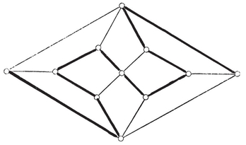
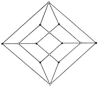
Fig. 1.5A shows a solution of this problem in a special caste 6 which is of interest as being the simplest instance where the journey cannot possibly be a “round trip”. Fig. 1.5B shows a map for which the problem is insoluble even if we are allowed to start from any one vertex and finish at any other.7
Although it is not always possible to include all the vertices of a polyhedron in a single chain of edges, it certainly is possible to include them all as nodes of a tree (whose N0–1 branches occur among the N1 edges). This merely requires repeated application of the principle that any two vertices may be connected by a chain of edges. In fact, every connected graph has a tree for its “scaffolding ” (Gerüst 8), and the connectivity of the graph is defined as the number of its branches that have to be removed to produce the tree, namely 1–N0+N1.
1·6. Euler’s Formula. In defining a polyhedron, we did not exclude the possibility of its being multiply-connected (i.e., ring-shaped, pretzel-shaped, or still more complicated). The special feature which distinguishes a simply-connected polyhedron is that every simple closed curve drawn on the surface can be shrunk, or that every circuit of edges bounds a region (consisting of one face or more). For such a polyhedron, the numbers of elements satisfy Euler’s Formula
1·61
which can be proved in a great variety of ways.9 The following proof is due to von Staudt.
Consider a tree whose nodes are the N0 vertices, and whose branches are N0–1 of the N1 edges (i.e., a scaffolding of the graph of vertices and edges). Instead of the remaining edges, take the corresponding edges of the dual map (as in Fig. 1.4A, where the selected edges are drawn in heavy lines). These edges of the dual map form a graph with N2 nodes, one inside each face of the polyhedron. Its branches are entirely separate from those of the tree. It is connected, since the only way in which one of its nodes could be inaccessible from another would be if a circuit of the tree came between, but a tree has no circuits. On the other hand, a circuit of the graph would decompose the surface into two separate parts, each containing some nodes of the tree, which is impossible. So in fact the graph is a second tree, and has N2–1 branches. But every edge of the polyhedron corresponds to a branch of one tree or the other. Hence
(N0–1) + (N2–1) = N1.
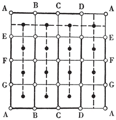
This argument breaks down for a multiply-connected surface, because there the graph of edges of the dual map does contain circuits (although these do not decompose the surface). For instance, the unbroken lines in Fig. 1.6A form the unfolded “ net ” of a map of sixteen quadrangles on a ring-shaped surface; the heavy lines form a scaffolding, and the broken lines cross the remaining edges. Two circuits of broken lines can be seen: one through the mid-point of AD, and another through the mid-point of AE.
Any orientable unbounded surface (e.g., any closed surface in ordinary space that does not cross itself) can be regarded as “a sphere with p handles ”. (Thus p=0 for a sphere or any simply-connected surface, p= 1 for a ring, and p=2 for the surface of a solid figure-of-eight.) The number p is called the genus of the surface. It can be shown10 that the appropriate generalization of 1•61 is
1·62
The unbroken lines in Fig. 1.4A· form a Schlegel diagram for the dodecahedron : one face is specialized, and the rest of the surface is represented in the interior of that face (as if we projected the polyhedron onto the plane of that face from a point just outside). Such a diagram can be made for any simply-connected polyhedron. 11We may regard the whole plane as representing the whole surface, by letting the exterior region of the plane represent the interior of the special face.
If a simply-connected map has only even faces (like Fig. 1.5A or B), we can show that every circuit of edges consists of an even number of edges. For, such a circuit, of (say) N edges, decomposes the map into two regions which have the circuit as their common boundary. If we modify the map, replacing one of the two regions by a single N-sided face, then the rest of the faces (belonging to the other region) are all even. Hence, by the remark at the end of § 1·4 N is even.
It follows that alternate vertices of any even-faced simply-connected map can be picked out in a consistent manner (so that every edge joins two vertices of opposite types). For instance, alternate vertices of a cube belong to two inscribed tetrahedra (Plate I, Fig. 6).
1·7. Regular maps. A map is said to be regular, of type {p, q}, if there are p vertices and p edges for each face, q edges and q faces at each vertex, arranged symmetrically in a sense that can be made precise.12 Thus a regular polyhedron (§ 1·3) is a special case of a regular map. By 1·41 and 1·44, we have
1·71
For each map of type {p, q} there is a dual map of type {q, p} ; e.g., a self-dual map of type {4, 4} is produced if we divide a torus or ring-surface into n2 “ squares ” by drawing n circles round the ring and n other circles threading the ring. (Fig. 1.6A shows the case when n=4. The surface has been cut along the circles ABCD and AEFG, one of each type.)
This example is ruled out if we restrict consideration to simply-connected polyhedra. Then the possible values of p and q are limited by the inequality 1•31, and for each admissible pair of values there is essentially only one polyhedron {p, q}. In fact, the relations 1•61 and 1•71 yield
1·72
which expresses N1 in terms of p and q. The inequality 1·31 is an obvious consequence of 1·72. The solutions
{3, 3}, {3, 4}, {4, 3}, {3, 5},
give the tetrahedron, octahedron, cube, icosahedron, dodecahedron. As maps we have also the dihedron {p, 2} and the hosohedron 13. The latter is formed by p digons or “ lunes.”
1·8. Configurations. A configuration in the plane is a set of N0 points and N1 lines, with N01 of the lines passing through each of the points, and N10 of the points lying on each of the lines. Clearly
N0 N01 = N1 N10.
For instance, N1 N01= 2 and N10 = N1−1. Again, a p-gon is a configuration in which N0 =N1=p, N01=N10=2. (Further points of intersection, of sides produced, are not counted.)
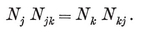
Analogously, a configuration in space is a set of N0 points, N1 lines, and N2 planes, or let us say briefly Nj j-spaces (j=0, 1, 2), where each j-space is incident with Njk of the k-spaces (j ≠ k).14 Clearly
1·81
These configurational numbers are conveniently tabulated as a matrix
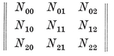
where Njj is the number previously called Nj.
The subject of configurations belongs essentially to projective geometry, in which the principle of duality enables us to preserve the relations of incidence after interchanging points and planes. Thus, for any configuration there is a dual configuration, whose matrix is derived from that of the given configuration by a “central inversion ” (replacing Njk by Nj′k′ where j + j′=k + k′= 2).
In particular, for each Platonic solid {p, q} we have a configuration
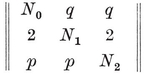
Here the relations 1.71 or 1.81 determine the ratios N0 : N1 : N2, and then 1.61 fixes the precise values
1·82

(See Table I, on page 292.)
1·9. Historical remarks. Sir D’Arcy W. Thompson once remarked to me that Euclid never dreamed of writing an Elementary Geometry : what Euclid really did was to write a very excellent (but somewhat long-winded) account of the Five Regular Solids, for the use of Initiates. However, this idea, first propounded by Proclus, is denied by Heath.
The early history of these polyhedra is lost in the shadows of antiquity. To ask who first constructed them is almost as futile as to ask who first used fire. The tetrahedron, cube and octahedron occur in nature as crystals15 (of various substances, such as sodium sulphantimoniate, common salt, and chrome alum, respectively). The two more complicated regular solids cannot form crystals, but need the spark of life for their natural occurrence. Haeckel observed them as skeletons of microscopic sea animals called radiolaria, the most perfect examples being Circogonia icosahedra and Circorrhegma dodecahedra.16 Turning now to mankind, excavations on Monte Loffa, near Padua, have revealed an Etruscan dodecahedron which shows that this figure was enjoyed as a toy at least 2500 years ago. So also to-day, an intelligent child who plays with regular polygons (cut out of paper or thin cardboard, with adhesive flaps to stick them together) can hardly fail to rediscover the Platonic solids. They were built up that “ childish ” way by Plato himself (about 400 B.C.) and probably before him by the earliest Pythagoreans, 17 one of whom, Timaeus of Locri, invented a mystical correspondence between the four easily constructed. solids (tetrahedron, octahedron, icosahedron, cube) and the four natural “ elements ” (fire, air, water, earth). Undeterred by the occurrence of a fifth solid, he regarded the dodecahedron as a shape that envelops the whole universe.
All five were treated mathematically by Theaetetus of Athens, and in Books XIII-XV of Euclid’s Elements ; e.g., 1.71 is Euclid XV, 6. (Books XIV and XV were not written by Euclid himself, but by several later authors.) The pyramids and prisms are much older, of course ; but antiprisms do not seem to have been recognized before Kepler (A.D. 1571-1630).18
The Greeks understood that some regular polygons can be constructed with ruler and compasses, while others cannot. This question was not cleared up until 1796, when Gauss, investigating the cyclotomic equation 1.15, concluded that the only {p}’s capable of such Euclidean construction are those for which the odd prime factors of p 19 means that p must be a divisor of
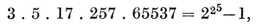
multiplied by any power of 2. The simplest rules for constructing {5} and {17} have been given by Dudeney and Richmond. Richelot and Schwendenwein constructed {257} about 1832, and J. Hermes wasted ten years of his life on {65537}. His manuscript is preserved in the University of Göttingen.
The theory of graphs (so named by Sylvester) began with Euler’s problem of the Bridges in Königsberg, and was developed by Cayley, Hamilton, Petersen, and others. Euler discovered his formula 1.61 in 1752. Sixty years later, Lhuilier noticed its failure when applied to multiply-connected polyhedra. The subject of Topology (or Analysis situs) was then pursued by Listing, Möbius, Riemann, Poincaré, and has accumulated a vast literature.
The theory of maps received a powerful stimulus from Guthrie’s problem of finding the smallest number of colours that will suffice for the colouring of every possible map. The question whether this number (for a simply-connected surface) is 4 or 5, has been investigated by Cayley, Kempe, Tait, Heawood, and others, but still remains unanswered. Evidently two colours suffice for the octahedron, three for the cube or the icosahedron, four for the tetrahedron or the dodecahedron.
The well-known figure of two perspective triangles with their centre and axis of perspective is a configurations (as defined in §1.8) with N0=N1=10 and N01=N10=3, first considered by Desargues in 1636. The use of a symbol such as {p, q} (for a regular polyhedron with p-gonal faces, q at each vertex) is due to Schläfli (4, p. 44), so we shall call it a “Schläfli symbol ”. The formulae 1.82 are his also.
[]
¶ CHAPTER II
REGULAR AND QUASI-REGULAR SOLIDS
THIS chapter opens with a new “ economical ” definition for regularity : a polyhedron is regular if its faces and vertex angles are all regular. In § 2·2 we see how {q, p} can be derived from {p, q} by reciprocation. Much use is made later of the self-reciprocal property
which is the number of sides of the skew polygon formed by certain edges (see § 2.6). The computation of metrical properties (in § 2.4) is facilitated by considering some auxiliary polyhedra which are not quite regular, but more than “ semi-regular,” so it is natural to call them “ quasi-regular.” §§ 2.7 and 2·8 deal with solids bounded by rhombs or other parallelograms ; these are described in such detail, not only for their intrinsic interest, but for use in Chapter XIII.
2·1. Regular polyhedra. The definition of regularity in § 1·3 involves three statements : regular faces, equal faces, equal solid angles. (Regular solid angles can then be deduced as a consequence.) All three statements are necessary. For : the triangular dipyramid formed by fusing two regular tetrahedra has equal, regular faces ; prisms and antiprisms of suitable altitude have regular faces and equal solid angles; and certain irregular tetrahedra, called disphenoids, have equal faces and equal solid angles. (To make a model of a disphenoid, cut out an acute-angled triangle and fold it along the joins of the mid-points of its sides. The disphenoid is said to be tetragonal or rhombic according as the triangle is isosceles or scalene.)
It is interesting to find that another definition, involving only two statements, is powerful enough to have the same effect : we shall see that regular faces and regular solid angles suffice. For simplicity, we replace the consideration of solid angles (which are rather troublesome) by that of vertex figures.20
The vertex figure at the vertex O of a polygon is the segment joining the mid-points of the two sides through O ; for a {p} of side 2l, this is a segment of length

(See the broken line in Fig. 1.1A on page 3.) The vertex figure at the vertex O of a polyhedron is the polygon whose sides are the vertex figures of all the faces that surround O ; thus its vertices are the mid-points of all the edges through O. For instance, the vertex figure of the cube (at any vertex) is a triangle.
Now, according to our revised definition, a polyhedron is regular if its faces and vertex figures are all regular.
Since the faces are regular, the edges must be all equal, of length 2l, say. Similarly, since the vertex figures are regular, the faces must be all equal ; for otherwise some pair of different faces would occur with a common vertex O, at which the vertex figure would have unequal sides, namely 2l cos π/p for two different values of p. Moreover, the dihedral angles (between pairs of adjacent faces) are all equal ; for, those occurring at any one vertex belong to a right pyramid whose base is the vertex figure. Each lateral face of this pyramid is an isosceles triangle with sides l, l, 2l cos π/p. The number of sides of the base cannot vary without altering the dihedral angle. Hence this number, say q, is the same for all vertices, and the vertex figures must be all equal.
We thus have the regular polyhedron {p, q}. Its face is a {p} of side 2l, and its vertex figure is a {q} of side 2l cos π/p.
We easily see that the perpendicular to the plane of a face at its centre will meet the perpendicular to the plane of a vertex figure at its centre in a point O3 which is the centre of three important spheres : the circum-sphere which passes through all the vertices (and the circum-circles of the faces), the mid-sphere which touches all the edges (and contains the in-circles of the faces), and the in-sphere which touches all the faces.21 Their respective radii 22 will be denoted by 0R, 1R, and 2R.
Let O2, be the centre of a face, O1 the mid-point of a side of this face, and O0 one end of that side. Since the triangle O*i* O*j* O*k* (i < j< k) is right-angled at O*j*, Pythagoras’ Theorem gives
2·11
2·2. Reciprocation. Consider the regular polyhedron {p, q}, with its N0 vertices, N1 edges, N2 faces. (See 1·82.) If we replace each edge by a perpendicular line touching the mid-sphere at the same point, we obtain the N1 edges of the reciprocal polyhedron {q, p}, which has N2 vertices and N0 faces. This process is, in fact, reciprocation with respect to the mid-sphere : the vertices and face-planes of {q, p} are the poles and polars of the face-planes and vertices of {p, q}.
Reciprocation with respect to another (concentric) sphere would yield a larger or smaller {q, p}. The mid-sphere is convenient to use, as having the same relationship to both polyhedra ; e.g., it reciprocates the tetrahedron {3, 3} into an equal {3, 3}. (See Plate I, Figs. 6-8.) Moreover, when we use the mid-sphere, the circum-circle of the vertex figure of {p, q} coincides with the in-circle of a face of {q, p}, and these two {q}’s are reciprocal with respect to that circle.
If properties of the reciprocal of a given polyhedron are distinguished by dashes, we have
2·21
for, each of these expressions is equal to the square of the radius of reciprocation. Hence this radius can be chosen so that 0R=0R′ and 2R=2R′; but then we shall not, in general, have also 1R=1R′.
This process of reciprocation can evidently be applied to any figure which has a recognizable “centre”. It agrees both with the topological duality that we defined for maps (§ 1-4) and with the projective duality that applies to configurations (§ 1·8).
2.3. Quasi-regular polyhedra. In the case when two regular polyhedra, {p, q} and {q, p N1 vertices, namely the mid-edge points of either {p, q} or {q, p}. Its faces consist of N0 {q}’s and N2 {p}’s, which are the vertex figures of {p, q} and {q, p}, respectively. There are 4 edges at each vertex, and so 2N1 edges altogether. Euler’s Formula is satisfied, as
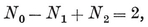
N1 − 2N1 + (N0 + N2) = 2.

When p=q=3, this derived polyhedron is evidently the octahedron ; for all its faces are {3}’s, and four meet at each vertex :
2·31
In other cases the {p}’s and {q}’s are different; but still the edges are all alike, each separating a {p} from a {q cuboctahedron,
 icosidodecahedron (Plate I, Figs. 9 and 10). These are instances (in fact, the only convex instances) of quasi-regular polyhedra.
A quasi-regular polyhedron is defined as having regular faces, while its vertex figures, though not regular, are cyclic and equiangular (i.e., inscriptible in circles and alternate-sided). It follows from this definition that the edges are all equal, say of length 2L, that the dihedral angles are all equal, and that the faces are of two kinds, each face of one kind being entirely surrounded by faces of the other kind. Moreover, by a natural extension of the argument used for a regular polyhedron in § 2·1, the vertex figures are all equal. If there are r {p}’s and r {q}’s at one vertex, then it is the same at every vertex, and the vertex figure is an equiangular 2r-gon with alternate sides 2L cos π/p and 2L cos π/q. The face-angles at a vertex make a total of
r(1 − 2/p)π + r(1 − 2/q)π,
which must be less than 2π ; therefore
2·32
But p and q cannot be less than 3; so r
On examining a model of the octahedron, cuboctahedron, or icosidodecahedron, we observe a number of equatorial r=2), and that either pair of opposite vertices of this rectangle are the mid-points of two adjacent sides of the equatorial polygon. If this polygon is an {h}, its vertex figure is of length 2L cos π/h. But this vertex figure, as we have just seen, is the diagonal of a rectangle of sides 2L cos π/p and 2L cos π/q. Hence
2·33
We can thus verify that h Fig. 2.3A.)
 h}; so there are 2N1/h such {h}’s altogether (namely 3 squares, 4 hexagons, and 6 decagons, in the respective cases).
The quasi-regular solids and their equatorial polygons
The equation 2-33 for h is useful in connection with trigonometrical formulae (such as those we shall find in § 2·4). But for other purposes it is desirable to have an algebraic expression for h. This can be found as follows. Since each of the 2N1/h equatorial h-gons meets each of the others at a pair of opposite vertices, we have
whence 4N1 = h(h + 2), and
2·34
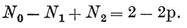
In virtue of 1·72, this is an algebraic expression for h in terms of p and q, as desired. Of course, it is not equivalent to 2-33 for general values of p and q, but only for the values corresponding to points (p, q) on the curve sketched in Fig. 2.3B, whose equation is obtained by eliminating h and N1 from 1·72, 2·33, 2·34. Part of this is the rectangular hyperbola
(p − 2)(q − 2) = 4,
corresponding to N1 = ∞ . But we are more interested in the other part, which contains the points (3, 5), (3, 4), (3, 3), (4, 3), (5, 3) corresponding to the Platonic solids {p, q}. The values of h are marked at these points. The two branches touch each other at two points where
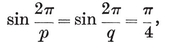
viz., (2·81, 6·96) and (6·96, 2·81). There is also an acnode at (2, 2), where h=2.
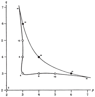
Values of p and q for which 2·33 and 2·34 agree
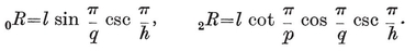
2.4. Radii and angles. The metrical properties of {p, q} can be expressed elegantly in terms of p, q, and h h} of side 2L, is L csc π/h
 p, q} of edge 2l, this circum-radius occurs as the mid-radius of {p, q}. But the edge 2L
 p, q}, namely 2l cos π/p. Hence
2·41

and the mid-radius of {p, q} is
2·42

It follows from 2·11 and 2·33 that the circum-radius and in-radius are
2·43
As a check, we observe that the ratio 0R/2R involves p and q symmetrically, in agreement with 2·21.
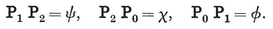
Let φ, χ, ψ denote the angles at O3 in the respective triangles O0 O1 O3, O0 O2 O3, O1 O2 O3, i.e., the angles subtended at the centre by a half-edge and by the circum- and in-radii of a face.23 Then the properties φ, χ, ψ of {p, q} are the properties ψ, χ, φ of {q, p} ; in fact,
2·44
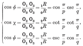
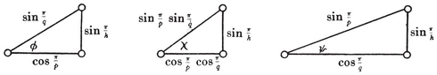
These and other trigonometrical functions of φ, χ, ψ may conveniently be read off from the right-angled triangles in Fig. 2.4A (which are similar to the triangles Oi Oj Ok). We observe also that
sin φ = l/0R,
and that π-2ψ is the dihedral angle between the planes of two adjacent faces. (This is easily seen by considering the section by the plane O1 O2 O3 which is perpendicular to the common edge of two such faces.)
The first of the formulae 2·44 expresses the fact that l cos φ is equal to the circum-radius of the vertex figure. This may alternatively be seen by considering the section of {p, q} by the plane O0 O1 O3 (joining one edge to the centre), as in Fig. 2.4B.
By 1·13 and 1·71, the surface-area of {p, q} is
2·45
where N1 is given by 1·72 or 1·82. The volume, being made up of N2 right pyramids of altitude 2R, is
2·46
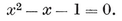
For the application of these formulae in the individual cases, see Table I on page 293, where frequent use has been made of the special number
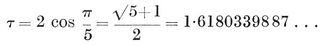
which is the positive root of the quadratic equation
2·47
Writing this equation as x=1+1/x, we see that
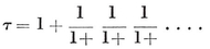
It is well known that, of all regular continued fractions, this converges slowest. Its nth convergent is fn+1/fn, where f1, f2, … are the Fibonacci numbers
1, 1, 2, 3, 5, 8, 13, 21, 34, 55, …
These can be written down immediately, as
1 + 1 = 2, 1 + 2 = 3, 2 + 3 = 5, 3 + 5 = 8,
and so on. Since τn−1 + τn = τn+1, the integral powers of τ are given by the formulae
e.g.,

2·5. Descartes’ Formula. In the deduction of 1·31 and 2·32, we used the principle that the face-angles at a vertex of a convex polyhedron must total less than 2π. It is evident to anyone making models, that the angular deficiency is small when the polyhedron is complicated. The precise connection was observed by Descartes, who showed that, if the face-angles at a vertex amount to 2π−δ, then
Σδ = 4π,
where the summation is taken over all the vertices.
If the vertices are all surrounded alike, this means that
2·51

i.e., the angular deficiency is inversely proportional to the number of vertices*. In the case of {p,* q*}, we have*
δ = 2π − q(1 − 2/p)π,
whence
N0 = 4p/(2p + 2q − pq),
in agreement with 1·82. If we measure δ in degrees, the formula is
N0 = 720/δ ;
e.g., the dodecahedron has three face-angles of 108°, totalling 324°, so the deficiency is 36°, and N0 = 720/36 = 20.
Descartes’ Formula is most easily established by spherical trigonometry, using the well-known fact that the area of a spherical triangle (whose sides are arcs of great circles on a sphere of unit radius) is equal to its spherical excess, which means the excess of its angle-sum over that of a plane triangle (namely π). Since any polygon can be dissected into triangles, it follows that the area of a spherical polygon is equal to its spherical excess, which means the excess of its angle-sum over that of a plane polygon having the same number of sides.
By projecting the edges of a given convex polyhedron from any interior point onto the unit sphere around that point, we obtain a partition of the sphere into N2 spherical polygons, one for each face of the polyhedron. The total angle-sum of all these polygons is clearly 2πN0 (i.e., 2π for each vertex). On the other hand, the total angle-sum of the flat faces themselves is
Σ (2π − δ) = 2πN0 − Σδ
(summed over the vertices). The difference, Σδ, is the total spherical excess of the N2 spherical polygons, which is the total area of the spherical surface, namely 4π.
Spherical trigonometry also facilitates the derivation of 2·44. For, by projecting the triangle O0 O1 O2 from the centre O3 onto the unit sphere around O3, we obtain a spherical triangle P0 P1 P2 with angles

and (opposite) sides
2·52
The ordinary formulae for a right-angled spherical triangle give 2·44 at once.
2·6. Petrie polygons p, q}. In particular, the vertices of an equatorial {h} are the mid-points of a special circuit of h edges of {p, q}, forming a skew polygon which is sufficiently important to deserve a name of its own : so let us call it a Petrie polygon. It may alternatively be defined as a skew polygon such that every two consecutive sides, but no three, belong to a face of the regular polyhedron. The above considerations show that it is a skew h-gon, where hhh-gonal antiprism. (See § 1·3, where the icosahedron {3, 5} was derived from a pentagonal antiprism by adding two pyramids.)
Fig. 2.3A h}’s. Fig. 2.6A shows the corresponding projections of {p, q}. The peripheries are still plane h-gons, but now they are the projections of skew h-gons, namely Petrie polygons.
 N1/h equatorial polygons. Hence the regular polyhedron {p, q} has 2N1/h Petrie polygons (all alike). The reciprocal polyhedron {q, p} has the same number of Petrie polygons ; but these have a different shape, unless p=q.
The Platonic solids and their Petrie polygons
2·7. The rhombic dodecahedron and triacontahedron. Consider once more the figure formed by solids {p, q} and {q, p N1 rhombs. The diagonals of these rhombs are the edges of {p, q} and {q, p}. The polyhedron is easily seen to have 2N1 edges and N0+N2
 24 When p=q
 rhombic dodecahedron and the triacontahedron (Plate I, Figs. 11 and 12). The former is shown by a Schlegel diagram in Fig. 1.5B.
The shape of the rhomb is determined by the fact that its diagonals are 2l and 2l’, where, by 2·41,
2·71

In particular, the face of the rhombic dodecahedron has diagonals in the ratio 1 : √2. This suggests an amusing method for building up a model.25 Take two equal solid cubes. Cut one of them into six square pyramids based on the six faces, with their common apex at the centre of the cube. Place these pyramids on the respective faces of the second cube. The resulting solid is the rhombic dodecahedron.
Alternatively,26 a model of the rhombic dodecahedron can be built up by juxtaposing four obtuse rhombohedra whose faces have diagonals in the ratio 1 : √2. (A rhombohedron is a parallelepiped bounded by six equal rhombs. It has two opposite vertices at which the three face-angles are equal. It is said to be acute or obtuse according to the nature of these angles.)
By 2·71 again, the triacontahedron’s face has diagonals in the “ golden section ” ratio 1 : τ. A model can be built up from twenty rhombohedra, ten acute and ten obtuse, bounded by such rhombs.27 (The thirty faces of the triacontahedron are accounted for as follows. Seven of the obtuse rhombohedra possess three each, and nine of the acute rhombohedra possess one each. The remaining four rhombohedra are entirely hidden in the interior.)
Corresponding to the equatorial h zone of h rhombs, encircling it like Humpty Dumpty’s cravat. The edges along which consecutive rhombs of the zone meet are, of course, all parallel. It follows that the dihedral angle of the “ rhombic N1-hedron ” is

i.e., 90° for the cube, 120° for the rhombic dodecahedron, and 144° for the triacontahedron.
2·8. Zonohedra. These rhombic figures suggest the general concept of a convex polyhedron bounded by parallelograms. We proceed to prove that such a polyhedron has n(n-1) faces, where n is the number of different directions in which edges occur.
Since all the faces are parallelograms, every edge determines a zone of faces, in which each face has two sides equal and parallel to the given edge. Every face belongs to two zones which cross each other at that face and again elsewhere (at the “ counterface ”). Hence the faces occur in opposite pairs which are congruent and similarly situated in parallel planes. So also, the edges occur in opposite pairs which are equal and parallel, and the vertices occur in opposite pairs whose joins all have the same mid-point. In other words, the polyhedron has central symmetry. Hence each zone crosses every other zone twice. If edges occur in n different directions, there are n zones, each containing n n directions there is a pair of faces whose sides occur in those directions. Thus there are n(n−1) faces. 28
Moreover, there are 2(n−1) edges in each direction : 2n(n−1) edges altogether. By 1·61, there are n(n−1)+2 vertices.
Let us define a star as a set of n line-segments with a common mid-point, and call it non-singular if no three of the lines are coplanar. Then we may say that every convex polyhedron bounded by parallelograms determines a non-singular star, having one line-segment for each set of 2(n−1) parallel edges of the polyhedron.
Conversely, the star determines the polyhedron. To see this, consider n vectors e1, e2, … , en, represented by the segments of the star (with a definite sense of direction chosen along each). The various sums of these vectors without repetition, say
2·81

will lead from a given point to a certain set of 2*n* points, not necessarily all distinct. The smallest convex body containing all these points (on its surface or inside) is a polyhedron whose edges represent the vectors ei in various positions. If the star is non-singular, the faces are parallelograms.
To see which sums of vectors lead to vertices, consider a plane of general position through a fixed point from which the vectors e1, . . . , en proceed in their chosen directions. The sum of those vectors which lie on one side of the plane is the vector leading to a vertex of the polyhedron ; the sum of the vectors on the other side leads to the opposite vertex. Hence the number of pairs of opposite vertices is equal to the number of ways in which the n vectors can be separated into two sets by a plane. By considering what happens in the plane at infinity, we can identify this with the number of ways in which n points in the real projective plane can be separated by a line. By the principle of duality, this is equal to the number of regions into which the plane is dissected by n lines. If the given star is non-singular, these n
Here are some simple instances : the general star with n=3 determines a parallelepiped ; and the star whose segments join opposite vertices of an octahedron, cube or icosahedron, determines a cube, rhombic dodecahedron or triacontahedron, respectively.
The analogous process in two dimensions leads from a star of n coplanar segments to a convex polygon which has central symmetry, its n pairs of opposite sides being equal and parallel to the n segments. Since such a flat star is a limiting case of a star of n non-coplanar segments, the “ parallel-sided 2n
The general star (wherein various sets of m lines are coplanar) leads to a convex polyhedron whose faces are parallel-sided 2m-gons (e.g., when m=2, parallelograms). This is the general zonohedron. By a natural extension of the above argument, we see that every convex polyhedron bounded by parallel-sided 2m-gons is a zonohedron. Hence, if every face of a convex polyhedron has central symmetry, so has the whole polyhedron.29
The expression n(n−1), for the number of parallelograms in a “ non-singular ” zonohedron, applies also to the general zonohedron, provided we regard each parallel-sided 2m
2·82
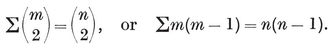
Plate II shows a collection of equilateral zonohedra, whose stars consist of equal segments. (The faces with m> 2 have been marked according to their dissection into rhombs, in various ways simultaneously. The reason for doing this will appear in § 13-8.)
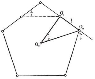
By removing one zone from the triacontahedron, and bringing together the two remaining pieces of the surface, we obtain the rhombic icosahedron, which has a decidedly “ oblate ” appearance. The corresponding star consists of five of the six diameters of the icosahedron, i.e., five segments joining pairs of opposite vertices of a pentagonal antiprism. More generally, the star which joins opposite vertices of any right regular n-gonal prism (n even) or antiprism (n odd) determines a polar zonohedron (Fig. 2.8A) whose faces consist of n equal rhombs surrounding one vertex, n other rhombs beyond these, and so on: n−1 sets of n rhombs altogether, ending with those that surround the opposite vertex.30
FIG. 2.8A : Polar zonohedra
Another special class of zonohedra consists of the five “ primary parallelohedra ”, each of which, with an infinity of equal and similarly situated replicas, would fill the whole of space without interstices.31 These are the cube, hexagonal prism, rhombic dodecahedron, “ elongated dodecahedron ” (Fig. 13.8B on page 257), and “truncated octahedron”. The last is bounded by six squares and eight hexagons ; its star consists of the six diameters of the cuboctahedron, and the corresponding lines in the real projective plane are the sides of a complete quadrangle (giving twelve regions).
2·9. Historical remarks. As long ago as 300 A.D., the unknown author of Euclid XV, 3-5, inscribed an octahedron in a cube, a cube in an octahedron, and a dodecahedron in an icosahedron ; this, in each case, amounts to reciprocating the latter solid with respect to its in-sphere (which is the circum-sphere of the former). He also inscribed an octahedron in a tetrahedron (Euclid XV, 2), thus anticipating 2·31. But Maurolycus (1494–1575) was probably the first to have a clear understanding of the relation between two reciprocal polyhedra.
The cuboctahedron and icosidodecahedron, described in § 2·3, are two of the thirteen Archimedean solids. Unfortunately, Archimedes’ own account of them is lost. According to Heron, Archimedes ascribed the cuboctahedron to Plato.32
The number of sides of the Petrie polygon of {p, q} is given by the alternative formulae 2·33 and 2·34, the latter of which is published here for the first time.33 When the general formulae of § 2·4 are applied to the individual polyhedra, as in Table I on page 293, the results are seen to agree with van Swinden 1, pp. 378-390. But some of these results are far older. Euclid himself found all the circum-radii (or, rather, their reciprocals, the edges of the solids inscribed in a given sphere ; see Euclid XIII, 18). Hypsicles (Euclid XIV) observed that, if a dodecahedron and an icosahedron have the same circum-sphere, they also have the same in-sphere,34 S/0R2 (or of C/0R3) for {p, q} and {q, p} are in the ratio
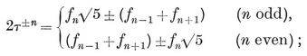
A line-segment is said to be divided according to the Golden Section if its two parts are in the ratio 1 : τ. (See 2·47.) A construction for this section was given by Eudoxus in the fourth century B.C. Since τ2=τ+1, the larger part and the whole segment are again in the ratio 1 : τ. In other words, a rectangle whose sides are in this ratio (viz., the vertex figure of the icosidodecahedron) has the property that, when a square is cut off, the remaining rectangle is similar to the original. The related sequence of integers was investigated in the thirteenth century A.D. by Leonardo of Pisa, alias Fibonacci.35 More recently, the remarkable formula
was discovered by Lucas (2, pp. 458, 463). It was Schläfli (4, p. 53) who first noticed the occurrence of various powers of τ in the metrical properties of the icosahedron and dodecahedron (and of other figures which we shall construct in Chapters VI, VIII, and XIV).
“ Descartes’ Formula ” (§ 2·5), which is practically an anticipation of Euler’s Formula (1·61), was discussed in a manuscript De Solidorum Elementis. This was lost for two centuries, and then turned up among the papers of Leibniz. 36
Meier Hirsch (1, p. 65) used spherical trigonometry in 1807 for his proof of the existence of the Platonic solids. The characteristic triangle P0 P1 P2 was used extensively by Hess (3, pp. 26-29).
The rhombic dodecahedron and triacontahedron (§ 2·7) were discovered by Kepler (1, p. 123) about 1611. The former occurs in nature as a garnet crystal, often as big as one’s fist. Strictly, it should be called the first rhombic dodecahedron, because in 1960 Bilinski (1) noticed that a second rhombic dodecahedron (whose faces have the same shape as those of the triacontahedron) can be derived from the rhombic icosahedron by removing one zone and bringing together the two remaining pieces of the surface.
§ 2·8 has the peculiarity of being concerned with affine geometry. The theory of zonohedra is due to the great Russian crystallographer Fedorov (1), who was particularly delighted with formula 2·82. He does not seem to have realized, however, that a convex zonohedron is capable of such a simple definition as this : a convex polyhedron whose faces are centrally symmetrical polygons.
John Flinders Petrie, who first realized the importance of the skew polygon that now bears his name, was the only son of Sir W. M. Flinders Petrie, the great Egyptologist. He was born in 1907, and as a schoolboy showed remarkable promise of mathematical ability. In periods of intense concentration he could answer questions about complicated four-dimensional figures by “ visualizing ” them. His skill as a draughtsman can be seen in his unique set of drawings of stellated icosahedra.37 In 1926, he generalized the concept of a regular skew polygon to that of a regular skew polyhedron.38 He worked for many years as a schoolmaster. In 1972, after a few months of retirement, he was killed by a car while attempting to cross a motorway near his home in Surrey.
PLATE II
SOME EQUILATERAL ZONOHEDRA
[]
¶ CHAPTER III
ROTATION GROUPS
THIS chapter provides an introduction to the theory of groups, illustrated by the symmetry groups of the Platonic solids. We shall find coordinates for the vertices of these solids, and examine the cases where one can be inscribed in another. Finally, we shall see that every finite group of displacements is the group of rotational symmetry operations of a regular polygon or polyhedron.
3·1. Congruent transformations. Two figures are said to be congruent if the distances between corresponding pairs of points are equal, in which case the angles between corresponding pairs of lines are likewise equal. In particular, two trihedra (or trihedral solid angles) are congruent if the three face-angles of one are equal to respective face-angles of the other. Two such trihedra are said to be directly congruent (or “ superposable ”) if they have the same sense (right- or left-handed), but enantiomorphous if they have opposite senses. The same distinction can be applied to figures of any kind, by the following device.
Any point P is located with reference to a given trihedron by its (oblique) Cartesian coordinates x, y, z. Let P’ be the point whose coordinates, referred to a congruent trihedron, are the same x, y, z. If we suppose the two trihedra to be fixed, every P determines a unique P′, and vice versa. This correspondence is called a congruent transformation, P′ being the transform of P. If another point Q is transformed into Q′, we have a definite formula for the distance PQ in terms of the coordinates, which shows that P′Q′=PQ. In other words, a congruent transformation is a point-to-point correspondence preserving distance. It is said to be direct or opposite according as the two trihedra are directly congruent or enantiomorphous, i.e., according as the transformation preserves or reverses sense. Hence the product (resultant) of two direct or two opposite transformations is direct, whereas the product of a direct transformation and an opposite transformation (in either order) is opposite. (In fact, the composition of direct and opposite transformations resembles the multiplication of positive and negative numbers, or the addition of even and odd numbers.) A direct transformation is often called a displacement, as it can be achieved by a rigid motion. Any two congruent figures are related by a congruent transformation, direct or opposite. Two identical left shoes are directly congruent ; a pair of shoes are enantiomorphous. (Some authors use the words “ congruent ” and “ symmetric ” where we use “ directly congruent ” and “ enantiomorphous ”.)
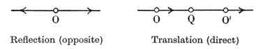
We shall find that all congruent transformations can be derived from three “ primitive ” transformations : translation (in a certain direction, through a certain distance), rotation (about a certain line or axis, through a certain angle), and reflection (in a certain plane). Evidently the first two are direct, while the third is opposite.
There is an analogous theory in space of any number of dimensions. In two dimensions we rotate about a point, reflect in a line, and a congruent transformation is defined in terms of two congruent angles. In one dimension we reflect in a point, and a congruent transformation is defined in terms of two rays (or “ half lines ”). In this simplest case, if any point O is left invariant, the transformation is the reflection in O, unless it is merely the identity (which leaves every point invariant) ; but if there is no invariant point, it is a translation, i.e., the product of reflections in two points (O and Q, in Fig. 3.1A).
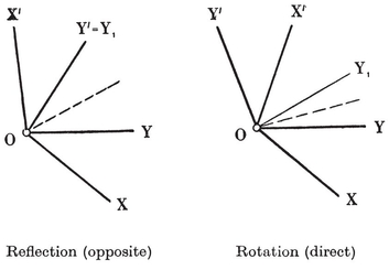
In two dimensions, a congruent transformation that leaves a point O invariant is either a reflection or a rotation (according as it is opposite or direct). For, the transformation from an angle XOY to a congruent angle X′OY′ (Fig. 3.1B) can be achieved as follows. By reflection in the bisector of ∠XOX′, ∠XOY is transformed into ∠X′OY1. Since this is congruent to ∠X′OY′, the ray OY’ either coincides with OY1 or is its image by reflection in OX′. In the former case the one reflection suffices ; in the latter, it has to be combined with the reflection in OX′, and the product is the rotation through ∠XOX′ (which is twice the angle between the two reflecting lines).
In particular, the product of reflections in two perpendicular lines is a rotation through π or half-turn. In this single case, it is immaterial which reflection is performed first ; in other words, two reflections commute if their lines are perpendicular. It is important to notice that the half-turn about O is the product of reflections in any two perpendicular lines through O.
A plane congruent transformation without any invariant point is the product of two or three reflections (according as it is direct or opposite). For, in transforming an angle XOY into a congruent angle X′O′Y′, we can begin by reflecting in the perpendicular bisector of OO′, and then use one or two further reflections, as above.
The product of two reflections is a translation or a rotation, according as the reflecting lines are parallel or intersect. Hence every plane displacement is either a translation or a rotation.39
In the product of three reflections, we can always arrange that one of the reflecting lines shall be perpendicular to both the others. The following is perhaps not the simplest proof, but it is one that generalizes easily to any number of dimensions. If we regard a congruent transformation as operating on pencils of parallel rays (instead of operating on points), we can say that a translation has no effect : it leaves every pencil invariant. Since each pencil can be represented by that one of its rays which passes through a fixed point O, any congruent transformation gives rise to an “ induced ” congruent transformation operating on the rays that emanate from O : congruent because of the preservation of angles.
If the given transformation is opposite, so is the induced transformation. But the latter, leaving O invariant, can only be a reflection, say the reflection in OQ. This leaves O and Q invariant; therefore the given transformation leaves the direction OQ invariant. Consider the product of the given transformation with the reflection in any line, p, perpendicular to OQ. This is a direct transformation which reverses the direction OQ; i.e., it is a half-turn. Hence the given transformation is the product of a half-turn with the reflection in p. But the half-turn is the product of reflections in two perpendicular lines, which may be chosen perpendicular and parallel to p. Thus we have altogether three reflections, of which the last two can be combined to form a translation. The general opposite transformation is now reduced to the product of a reflection and a translation which commute, the reflecting line being in the direction of the translation. This kind of transformation is called a glide-reflection.
In three dimensions, a congruent transformation that leaves a point O invariant is the product of at most three reflections : one to bring together the two x-axes, another for the y-axes, and a third (if necessary) for the z-axes. Since one further reflection will suffice to bring together two different origins (i.e., the vertices of the two congruent trihedra),
3·11. Every congruent transformation is the product of at most four reflections*.*
Since the product of two opposite transformations is direct, a product of reflections is direct or opposite according as the number of reflections is even or odd. Hence every direct transformation is the product of two or four reflections, and every opposite transformation is either a single reflection or a product of three.
The product of reflections in two parallel planes is a translation in the perpendicular direction through twice the distance between the planes, and the product of reflections in two intersecting planes is a rotation about the line of intersection through twice the angle between them. Two reflections commute if their planes are perpendicular, in which case their product is a half-turn (or “ reflection in a line ”).
Since the product of three reflections is opposite, a direct transformation with an invariant point O can only be the product of reflections in two planes through O, i.e., a rotation. Thus
3·12. Every displacement leaving one point invariant is a rotation*.40*
Consequently the product of two rotations with intersecting axes is another rotation.
The three “ primitive ” transformations (viz., translation, rotation, and reflection), taken in commutative pairs, form the following three products. A screw-displacement is a rotation combined with a translation in the axial direction. A glide-reflection is a reflection combined with a translation whose direction is that of a line lying in the reflecting plane. A rotatory-reflection is a rotation combined with the reflection in a plane perpendicular to the axis. In the last case, if the rotation is a half-turn, the rotatory-reflection is an inversion (or “ reflection in a point ”), and the direction of the axis is indeterminate. In fact, an inversion is the product of reflections in any three perpendicular planes through its centre ; e.g., reflections in the axial planes of a Cartesian frame reverse the signs of x, y, z, respectively, and their product transforms (x, y, z) into (–x,–y,–z).
We proceed to prove that every congruent transformation is of one of the above kinds.
An opposite transformation, being the product of (at most) three reflections, leaves invariant either a point or two parallel planes (and all planes parallel to them). The latter possibility is the limiting case of the former when the invariant point recedes to infinity ; it arises when the three reflecting planes are all perpendicular to one plane, instead of forming a trihedron.
If there is an invariant point O, consider the product of the given (opposite) transformation with the inversion in O. This direct transformation, leaving O invariant, must be a rotation. Hence the given transformation is a “rotatory-inversion”, the product of a rotation with the inversion in a point on its axis. By regarding the inversion as a special rotatory-reflection,41 we see that a rotatory-inversion involving rotation through angle θ is the same as a rotatory-reflection involving rotation through θ–π. Hence every opposite transformation leaving one point invariant is a rotatory-reflection.
If, on the other hand, it is two parallel planes that are invariant, the transformation is essentially two-dimensional : what happens in one of the two planes happens also in the other and in all parallel planes. By the two-dimensional theory, we then have a glide-reflection. Hence
3·13. Every opposite congruent transformation is either a rotatory-reflection or a glide-reflection (including a pure reflection as a special case).
In order to analyse the general displacement or direct transformation, we first regard the transformation as operating on bundles of parallel rays, represented by single rays through a fixed point O. The induced transformation, leaving O invariant, is still direct, and so can only be a rotation. The direction of the axis, OQOQ.OQ,OQ with a translation in the direction OQ (or QO), i.e., a screw-displacement. Hence
3.14. Every displacement is a screw-displacement (including, in particular, a rotation or a translation).42
3.2. Transformations in general. The concept of a congruent transformation, applied to figures in space, can be generalized to that of a one-to-one transformation applied to any set of elements. 43 When we speak of the resultant of two transformations as their “ product ”, we are making use of the analogy that exists between transformations and numbers. We shall often use letters R, S, … to denote transformations, and write RS for the resultant of R and S (in that order). This notation is justified by the validity of the associative law
3·21
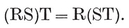
Since a number is unchanged when multiplied by 1, it is natural to use the same symbol 1 for the “ identical transformation ” or identity (which enters our discussion as the translation through no distance, and again as the rotation through angle 0 or through a complete turn). Pushing the analogy farther, we let R*p* denote the p-fold application of R; e.g., if R is a rotation through θ, R*p* is the rotation through pθ about the same axis. A transformation R is said to be periodic if there is a positive integer p such that R*p*=1; then its period is the smallest p for which this happens. We also let R−1 denote the inverse of R, which neutralizes the effect of R, so that RR−1= 1 = R−1R. If R is of period p, we have R−1=R*p*−1. In particular, a transformation of period 2 (such as a reflection, half-turn, or inversion) is its own inverse.
The general formula for the inverse of a product is easily seen to be
(RS . . . T)−1= T−1 . . . S−1 R−1.
If R, etc. are of period 2, this is the same as T … SR ; e.g., if R and S are reflections in parallel planes, the products RS and SR are two inverse translations, proceeding in opposite directions. The analogy with numbers might be regarded as breaking down in the general failure of the commutative law SR=RS ; but there are generalized numbers, such as quaternions, which likewise need not commute.
Let x denote any figure to which a transformation is applied. If T transforms x into x′ (so that T−1 transforms x into x′), we write x′ = xT.
x′ = x**T.**
This notation is justified by the fact that (xT)S=xTS. If S transforms the pair of figures (x, xT) into (x1;T into T1, and write
T1 = Ts.
(We may speak of this as “ T transformed by S ” ; e.g., if T is a rotation about an axis 1, then Ts is the rotation through the same angle about the transformed axis Is.) Since x1=xs x. Hence ST1=TS, and
TS = S−1TS.
Transforming a product, we find that
(TU)S = S−1TUS = S−1TSS−1US = TSUs.
Hence, for any integer p, (T*p)s = (Ts)p*.
If S and T commute, so that TS=ST and TS=T, we say that T is invariant under transformation by S.
The “ figure ” x need not be geometrical ; e.g., it could be a number or variable, in which case xT is a function of this variable, and a more customary notation is T(x). (The particular transformations
x′ = x*t*,
where t takes various numerical values, are seen to combine among themselves just like the numbers t.) Again, x could be a discrete set of objects in assigned positions, and xT the same set rearranged; then T is a permutation.
The two alternative notations currently used for permutations are illustrated by the symbols
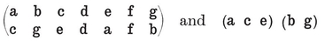
for the permutation of seven letters that replaces a**, b, c, e, g,** by c, g, e, a, b, while leaving d and f unchanged. In the latter notation, which we shall use exclusively, the two parts (a c e) and (b g) are called cycles. Clearly, every permutation is a product of cycles involving distinct sets of objects. It is sometimes desirable to include all the objects, e.g., to write
(a c e) (b g) (d) (f),
calling (d) and (f) “ cycles of period 1 ”. A transposition is a single cycle of period 2, such as (b g), which merely interchanges two of the objects.
A permutation is said to be even or odd according to the parity of the number of cycles of even period ; e.g., (a c e) (b g) is an odd permutation. When a permutation is multiplied by a transposition, its parity is reversed. For, if (a1 b1) is the transposition, a1 and b1 must either occur in the same cycle of the given permutation or in two different cycles. Since and
it merely remains to observe that one or all of the three periods r, s, r+s must be even.44 It follows (by induction) that every product of an even [odd] number of transpositions is an even [odd] permutation.
[image]{.image .placeholder original-image-src=“content/images/00114” original-image-title=“” width=“0in” height=“0in”} The subject of group-theory has been adequately expounded many times, so we shall be content to recall just the most relevant of its topics, in an attempt to make this book reasonably self-contained.
A set of elements or “ operations ” is said to form an abstract group if it is closed with respect to some kind of associative “multiplication”, if it contains an “identity”, and if each operation has an “inverse”. More precisely, a group contains, for every two of its operations R and S, their product RS ; [image]{.image .placeholder original-image-src=“content/images/00114” original-image-title=“” width=“0in” height=“0in”} holds for all R, S, T ; there is an identity, 1, such that
1R=R
for all R ; and each R has an inverse, R−1, such that
R−1R = 1.
It is then easily deduced that R1 = R and RR−1= 1.
The number of distinct operations (including the identity) is called the order of the group. This is not necessarily finite.
A subset whose products (with repetitions) comprise the whole group is called a set of generators (as these operations “generate” the group). In particular, a single operation R generates a group which consists of all the powers of R, including R0=1. This is called a cyclic group ; it is finite if R is periodic, and then its order is equal to the period of R. We may say that the cyclic group of order p is defined by the relation
R*p* = 1,
with the tacit understanding that R*n≠*1 for 0<n<p. More generally, any group is defined by a suitable set of generating relations; e.g., the relations
[image]
define a group of order 6 whose operations are 1, R1, R2, R1 R2, R2 R1, and R1 R2 R1=R2 R1 R2.
A subset which itself forms a group is called a subgroup. (For the sake of completeness it is customary to include among the subgroups the whole group itself and the group of order one consisting of 1 alone.) In particular, each operation of any group generates a cyclic subgroup.
If a given subgroup consists of T1, T2, . . . , while S is any operation in the group, the set of operations ST*i* is called a left coset of the subgroup, and the set T*i*S is called a right coset.45 It can be proved that any two left (or right) cosets have either the same members or entirely different members. Hence the subgroup effects a distribution of all the operations in the group into a certain number of entirely distinct left (or right) cosets. This number is called the index of the subgroup. When the group is finite, the index is the quotient of the orders of the group and subgroup.
Two operations T and T′ are said to be conjugate if one can be transformed into the other, i.e., if the group contains an operation S such that T′=Ts, or ST′=TS. The relation of conjugacy is easily seen to be reflexive, symmetric, and transitive. A subgroup T1, T2, … is said to be self-conjugate if, for every S in the group, the operations T*i* are a permutation of their transforms T*is, i.e., if the left and right cosets STi* and T*j*S are identical (apart from order of arrangement of members). In particular, any subgroup of index 2 is self-conjugate.
If two groups, G1 and G2, have no common operations except the identity, and if each operation of G1 commutes with each operation of G2, then the group generated by G1 and G2 is called their direct product, G1 × G2. (This clearly contains G1 and G2 as self-conjugate subgroups.) For instance, the cyclic group of order pq, where p and q are co-prime, is the direct product of cyclic groups of orders p and q (generated by R*q* and R*p*, if R generates the whole group).
When the operations are interpreted as transformations, we have a representation of the abstract group as a transformation group.[image]{.image .placeholder original-image-src=“content/images/00114” original-image-title=“” width=“0in” height=“0in”}n objects ; it is then called a permutation group of degree n. A permutation group is said to be transitive (on the n objects) if its operations suffice to replace one object by all the others in turn. The three most important transitive groups are :
(i) the symmetric group of order n!, which consists of all the permutations of the n objects,
(ii) the alternating group of order n!/2, which consists of the even permutations,
(iii) the cyclic group of order n, which consists of the cyclic permutations, viz., the powers of the cycle (a1, … a*n*).
We easily verify that the alternating group is a subgroup of index 2 in the symmetric group (of the same degree). When n=2, (i) and (iii) are the same. When n=3, (ii) and (iii) are the same.
The six operations of the symmetric group on a, b, c are
[image]

In terms of the two generators R1=(a b) and R2=(a c), these are
1, R1, R2, R1 R2 R1, R1 R2, R2 R1.
It is instructive to compare this with the group consisting of the following six transformations of a variable x:

Two such groups are said to be isomorphic, because they have the same “ multiplication table ” and consequently both represent the same abstract group.46[image]
Let a group G contain a self-conjugate subgroup T. Then any operation S of G occurs in a definite coset 〈S〉 = ST = TS. The distinct cosets can be regarded as the operations of another group, in which products, identity, and inverse are defined by
〈R〉 〈S〉 = 〈RS〉 〈1〉 = T, 〈S〉−1 = 〈S−1〉.
This new group is called a factor group of G, or more explicitly the quotient group G/T. If it is finite, its order is equal to the index of T in G.
It may happen that G contains a subgroup S whose operations S*j* “ represent ” the cosets of T, in the sense that the distinct cosets are precisely 〈S*j*〉. Then S is isomorphic with G/T. For instance, if G[image]{.image .placeholder original-image-src=“content/images/00114” original-image-title=“” width=“0in” height=“0in”}T is the cyclic subgroup generated by R1 R2, then S could consist of 1 and R1. Again, if G is the continuous group of all displacements, while G/T is the same group regarded as “ operating on bundles of parallel rays ” (see page 38), then T is the group of all translations, and S is the group of rotations leaving one point invariant.
It may happen, further, that the subgroup S is self-conjugate, like T. Then T*i* Sj=Sj T*i*, and G = S × T. For instance, if G is the cyclic group of order 6 defined by R6=1, S and T might be the cyclic subgroups generated by R2 and R3, respectively.
[image]{.image .placeholder original-image-src=“content/images/00114” original-image-title=“” width=“0in” height=“0in”}[image]{.image .placeholder original-image-src=“content/images/00114” original-image-title=“” width=“0in” height=“0in”}symmetry operation. Clearly, all the symmetry operations of a figure together form a group (provided we include the identity). This is called the symmetry group of the figure.
Conversely, given a group of congruent transformations, we can construct a symmetrical figure by taking all the transforms of any one point. The group is a subgroup of the symmetry group of the figure ; in fact, it is usually the whole symmetry group. If the given group is finite, the figure consists of a finite number of points which the transformations permute. These points have a centroid (or “ centre of gravity ”) which is transformed into itself. Thus
[image]{.image .placeholder original-image-src=“content/images/00114” original-image-title=“” width=“0in” height=“0in”} Every finite group of congruent transformations leaves at least one point invariant.47
It follows that the transforms of any point by such a group lie on a sphere.
A group of transformations may be discrete without being finite. This means that every point has a discrete set of transforms, i.e., that any given point has a neighbourhood containing none of its transforms (save the given point itself).
In the case of the cyclic group generated by a single congruent transformation S, the transforms of a point A0 of general position are
. . . , A−2, A−1, A1, A2, … ,
 regular polygon[image]
The various kinds of congruent transformation lead to various kinds of polygon. If S is a reflection, half-turn, or inversion, the polygon reduces to a digon, {2}. If S is a rotation, the sides are equal chords of a circle ; if the angle of rotation is 2π/p, we have the ordinary regular polygon, {p}. (The case where p[image]{.image .placeholder original-image-src=“content/images/00114” original-image-title=“” width=“0in” height=“0in”}p becomes infinite : a sequence of equal segments of one line, the apeirogon, {∞}. If S is a glide-reflection, the “ polygon ” is a plane zigzag. If S is a rotatory-reflection, it is a skew zigzag, whose vertices lie alternately on two equal circles in parallel planes ; if the angle of the component rotation is π/p, the sides are the lateral edges of a p-gonal antiprism. (Cases where p=[image]{.image .placeholder original-image-src=“content/images/00114” original-image-title=“” width=“0in” height=“0in”}helical polygon, whose sides are equal chords of a helix.
In every case except that of the digon, the cyclic group generated by S is not the whole symmetry group of the generalized polygon ; e.g., there is a symmetry operation interchanging A*n* and A−*n* for all values of n (simultaneously). In the case of the ordinary polygon {p}, the line joining the centre to any vertex, or to the mid-point of any side, contains one other vertex or mid-side point ; thus there are p such lines. The p-gon is symmetrical by a half-turn about any of them, besides being symmetrical by rotation through any multiple of 2π/p about the “ axis ” of the polygon. Thus the complete symmetry group of {p} is of order 2p, consisting of p half-turns about concurrent lines in the plane of the polygon, and p rotations through various angles about one line perpendicular to that plane.
The symmetry operations of a figure are either all direct, or half direct and half opposite. For, if an opposite operation occurs, its products with all the direct operations are all the opposite operations. Thus the rotation group formed by the direct operations is either the whole symmetry group or a subgroup of index 2. In the latter case the opposite operations form the single distinct coset of this subgroup.
The complete symmetry group of {p}, as described above, is the rotation group of the dihedron {p[image]{.image .placeholder original-image-src=“content/images/00114” original-image-title=“” width=“0in” height=“0in”}dihedral group of order 2p. On the other hand, the complete symmetry group of {p, 2} is of order 4p, as it contains also the same rotations multiplied by the reflection that interchanges the two faces of the dihedron. As a symmetry operation of {p} itself, the reflection in its own plane does not differ from the identity. Thus the p half-turns can be replaced by their products with this reflection, which are reflections in p coaxial planes.
The situation becomes clearer when we take a purely two-dimensional standpoint, considering rotations about points and reflections in lines. Then the symmetry group of {p} consists of p reflections (in lines joining the centre to the vertices and mid-side points) and p rotations (about the centre) ; but the rotation group of {p} is cyclic.
It is interesting to observe that the dihedral group of order 6 (or “ trigonal dihedral group ”) is isomorphic with the symmetric group of degree 3. In fact, the six symmetry operations of the equilateral triangle {3} permute the vertices a, b, c[image]{.image .placeholder original-image-src=“content/images/00114” original-image-title=“” width=“0in” height=“0in”}Fig. 3.4A). The transpositions appear as reflections, and the cyclic permutations as rotations.

[image]{.image .placeholder original-image-src=“content/images/00114” original-image-title=“” width=“0in” height=“0in”}. The most interesting finite groups of rotations are the rotation groups of the regular polyhedra, which we proceed to investigate.
Every rotation that occurs in a finite group is of finite period ; so its angle must be commensurable with π. In fact, the smallest angle of rotation about a given axis is a submultiple of 2π, and all other angles of rotation about the same axis are multiples of this smallest one. For,48 if j and p are co-prime, we can find a multiple of j/p which differs from 1/p by an integer ; so if 2πj/p is the smallest angle of rotation that occurs, we must have j=1. The rotations about this axis then form a cyclic group of order p, so we speak of an axis of p-fold rotation. When p=2, 3, 4, or 5, the axis is said to be digonal, trigonal, tetragonal, or pentagonal.
Two reciprocal polyhedra obviously have the same symmetry group, and likewise the same rotation group. The centre of {p, q} is joined to the vertices, mid-edge points, and centres of faces, by axes of q-fold, 2-fold, and p-fold rotation. Clearly, no further axes of rotation can occur. In other words, the direct symmetry operations of the polyhedron consist of rotations through angles 2kπ/q, π, and 2jπ/p, about these respective lines. If we exclude the identity, these rotations involve q−1 values for k, and p−1 for j. But the vertices, mid-edge points, and face-centres occur in antipodal pairs. (In the case of the tetrahedron, each vertex is opposite to a face.) Hence the total number of rotations, excluding the identity, is

[image]{.image .placeholder original-image-src=“content/images/00114” original-image-title=“” width=“0in” height=“0in”}the order of the rotation group is 2N*1.*
The same result may also be seen as follows. Let a sense of direction be assigned to a particular edge. Then a rotational symmetry operation is determined by its effect on this directed edge. Thus there is one such rotation for each edge, directed in either sense : 2N1
In particular, we have the tetrahedral group of order 12, the octahedral group of order 24 (which is also the rotation group of the cube) and the icosahedral[image]
[image]{.image .placeholder original-image-src=“content/images/00114” original-image-title=“” width=“0in” height=“0in”}. We define a compound polyhedron (or, briefly, a compound) as a set of equal regular polyhedra with a common centre. The compound is said to be vertex-regular if the vertices of its components are together the vertices of a single regular polyhedron, and face-regular if the face-planes of its components are the face-planes of a single regular polyhedron. For instance, the diagonals of the faces of a cube are the edges of two reciprocal tetrahedra. (See Plate I, Fig. 6, or Plate III, Fig. 5.) These form a compound, Kepler’s stella octangula, which is both vertex-regular and face-regular : its vertices belong to a cube, and its face-planes to an octahedron.
We shall find it convenient to have a definite notation for compounds.49 If d distinct {p, q}’s together have the vertices of {m, n}, each counted c times, or the faces of {s, t}, each counted e times, or both, we denote the compound by
c{m, n}[d{p, q}] or [d{p, q}]e{s,t} or c{m, n}[d{p, q}]e{s,t}.
The reciprocal compound is clearly
[d{q, p}]c{n, m} or e{t, s}[d{q,p}] or e{t,s}[d{q, p}]c{n, m}.
The numbers of vertices of {m, n} and {p, q} are in the ratio d : c, and the numbers of faces of {s, t} and {p, q} are in the ratio d : e. For instance, the stella octangula is
{4, 3}[2]
(with c=e=1). Other examples will be obtained in the course of the following investigation of the polyhedral groups.
In order to identify the tetrahedral group with the alternating group of degree 4, we observe that the vertices of a regular tetrahedron are four points whose six mutual distances are all equal.
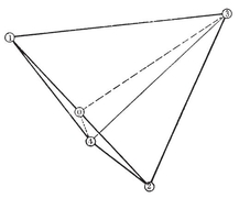
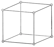
This statement involves the four points symmetrically, so we should expect all the 24 permutations in the symmetric group to be represented by symmetry operations of the tetrahedron. In fact, the transposition (1 2) is represented by the reflection in the plane 034, where 0 is the mid-point of the edge 12 (Fig. 3.6A). But any even permutation, being the product of two transpositions, is represented by a rotation. Thus the “ tetrahedral group ” (which we have defined as consisting of rotations alone) is the alternating group of degree 4.
PLATE III
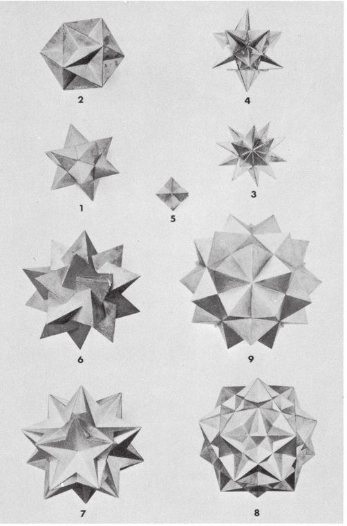
REGULAR STAR-YOLYHEDRA AND COMPOUNDS
In the stella octangula, every symmetry operation of either tetrahedron is also a symmetry operation of the cube ; but the cube has additional operations which interchange the two tetrahedra. The rotation group of the tetrahedron 1234 evenly permutes the four diameters 11′, 22′, 33′, 44′ of the cube (Fig. 3.6B). But the odd permutations of these diameters likewise occur as rotations ; e.g., 11′ and 22′ are transposed by a half-turn about the join of the mid-points of the two edges 12′ and 21′. Hence the octahedral group (which is the rotation group of the cube) is the symmetric group of degree 4.
If ABCDE and AEFGH are two adjacent faces of a regular dodecahedron, the vertices BDFH clearly form a square, whose sides join alternate vertices of pentagons. Moreover, these four vertices, with their antipodes, form a cube ; and alternate vertices of this cube form a tetrahedron (such as 1111 in Fig. 3.6C or D). It is easily seen that the rotations of this tetrahedron into itself are symmetry operations of the whole dodecahedron, i.e., that the tetrahedral group occurs as a subgroup in the icosahedral group (as well as in the octahedral group). The remaining operations of the icosahedral group transform this tetrahedron into others of the same sort, making altogether a compound of five tetrahedra inscribed in the dodecahedron. (Plate III, Fig. 6.) In other words, the twenty vertices of the dodecahedron are distributed in sets of four among five tetrahedra. The central inversion transforms this into a second compound of five tetrahedra, enantiomorphous (and reciprocal) to the first. The two together form a compound of ten tetrahedra (Fig. 7), reciprocal pairs of which can be replaced by five cubes (Fig. 8). Here each vertex of the dodecahedron belongs to two of the tetrahedra, and to two of the cubes.
We have thus obtained three vertex-regular compounds whose vertices belong to a dodecahedron. By reciprocation, we find that the compounds of tetrahedra are also face-regular, their face-planes belonging to an icosahedron. But the face-planes of the five cubes belong to a triacontahedron, so the reciprocal is a face-regular compound of five octahedra whose vertices belong to an icosidodecahedron. (Plate III, Fig. 9.) The appropriate symbols are :
{5, 3)[5]{3, 5},
2 [10]2,
2[5] and [5]2.
A very pretty effect is obtained by making models of these compounds, with a different colour for each component. The colouring of the five cubes determines a colouring of the triacontahedron in five colours, so that each face and its four neighbours have different colours. This scheme is used by Kowalewski as an aid to his Bauspiel[image]
The two enantiomorphous compounds of five tetrahedra may be distinguished as laevo and dextro. They provide a convenient symbolism for the twenty vertices of the dodecahedron (or for the twenty faces of the icosahedron) as follows. We number the five tetrahedra of the laevo compound as in Fig. 3.6C; those of the dextro compound (Fig. 3.6D) acquire the same numbers by means of the central inversion. Then the vertices of the dodecahedron are denoted by the twenty ordered pairs 12, 21, 13, 31, … , 45, 54, in such a way that ij is a vertex of the ith laevo tetrahedron and of the jth dextro tetrahedron. (For simplicity, the dodecahedron in Fig. 3.6E has been drawn as an opaque solid. The symbols for the hidden vertices are easily supplied, as ji is antipodal to ij.)
Each direct symmetry operation of the dodecahedron is representable as a permutation of the five digits ; e.g., the permutation (1 2 3) is a trigonal rotation about the diameter joining the opposite vertices 45 and 54, (1 4)(3 5) is a digonal rotation about the join of the mid-points of edges 13 45 and 31 54, and (1 2 3 4 5) is a pentagonal rotation about the join of centres of two opposite faces. Since all these are even permutations, we have proved that the icosahedral group is the alternating group of degree 5.
To sum up, the symmetric groups of degrees 3 and 4 are the rotation groups of {3, 2} and {3, 4}, and the alternating groups of degrees 4 and 5 are the rotation groups of {3, 3} and {3, 5}.
[image]{.image .placeholder original-image-src=“content/images/00114” original-image-title=“” width=“0in” height=“0in”}. The only regular polyhedron whose faces can be coloured alternately white and black, like a chess board, is the octahedron {3, 4}. For, this is the only polyhedron {p, q} with q even. In Fig. 3.6B we denoted the vertices of the cube by 1, 2, 3, 4, 1′, 2′, 3′, 4′. By reciprocation, the same symbols can be used for the faces of the octahedron, and we may distinguish the two sets of four faces as white and black. (In other words, we colour the faces of the octahedron like those of a stella octangula whose two tetrahedra are white and black, respectively.) By assigning a clockwise sense of rotation to each white face, and a counterclockwise sense to each black face, we obtain a coherent indexing of the edges, such as can be indicated by marking an arrow along each edge. Then, if we proceed along an edge in the indicated direction, there will be a white face on our right side and a black face on our left.
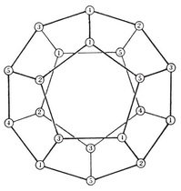

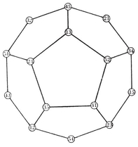
This enables us to define, for any given ratio a : b, twelve points dividing the respective edges in this ratio, so that the three points in each face form an equilateral triangle. In general, these twelve points will be the vertices of an irregular icosahedron, whose faces consist of eight such equilateral triangles and twelve isosceles triangles. Without loss of generality, we may suppose that a≥b. When a/b is large, the isosceles triangles have short bases ; in the limit they disappear, as their equal sides coincide and lie along the twelve edges of the octahedron. But when a approaches equality with b, the isosceles triangles tend to become right-angled ; in the limit, pairs of them form halves of the six square faces of a cuboctahedron, as in Fig. 8.4A on page 152.50 By considerations of continuity, we see that at some intermediate stage the isosceles triangles must become equilateral, and the icosahedron regular. In fact, the squares of the respective sides are a2−ab+b2 and 2b2, which are equal if
a2 − ab − b2 = 0,
so that a/b=τ.[image]{.image .placeholder original-image-src=“content/images/00114” original-image-title=“” width=“0in” height=“0in”}the twelve vertices of the icosahedron can be obtained by dividing the twelve edges of an octahedron according to the golden section. 51 For a given icosahedron, the octahedron may be any one of the [5]2.
In terms of rectangular Cartesian coordinates, the vertices of a cube (of edge 2) are
[image]
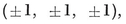
those of a tetrahedron (of edge 2√2) are
[image]

and those of an octahedron (of edge √2) are
[image]

If a+*b=*1, the segment joining (0, 0, 1) and (0, 1, 0) is divided in the ratio a : b by the point (0, a, b[image]
(0, ± a, ± b), (±b, 0, ±a), (±a, ±b, 0).
Hence the vertices of a cuboctahedron (of edge √2) are
[image]

and the vertices of an icosahedron (of edge 2) are
[image]

The planes of the faces
(0, τ, 1) (±1, 0, τ) and (0, τ, 1) (1, 0, τ) (τ, 1, 0)
are respectively
τ−1y + τz = τ2 and x + y + z = τ2.
(Remember that τ2= τ + 1.) Hence the vertices of the reciprocal dodecahedron (of edge 2τ–1) are
3·76

One of the five inscribed cubes is thus made very evident.
The mid-point of the edge (τ, ±1, 0) of the icosahedron 3·75 is (τ, 0, 0), while that of the edge (1, 0, τ) (τ τ−1) the vertices of an icosidodecahedron (of edge 2τ−1) are
3·77
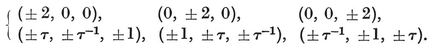
The vertices in the upper row belong to one of the octahedra of [5 {3, 4}]2.
3·8. The complete enumeration of finite rotation groups. In §§ 3·4 and 3·5 we considered various groups of rotations : cyclic, dihedral, tetrahedral, octahedral, icosahedral. The question now arises, Are these the only finite groups of rotations ? If so, they are also the only finite groups of displacements (by 3·41 and 3·12). We shall find that the answer is Yes.
Consider the general finite group of rotations. Since there is an invariant point O (lying on the axes of all the rotations), it is convenient to regard the group as operating on a sphere with centre O, instead of the whole space. Each rotation, having for axis a diameter of the sphere, is then regarded as a rotation about a point on the sphere. (We must remember, however, that the rotation through angle θ about any point is the same as the rotation through − θ about the antipodal point.) We saw (as a consequence of 3·12) that the product of two such rotations is another. To determine the product of two given rotations, we make use of the following theorem :
If the vertices of a spherical triangle PQR (like the triangle PQ1R in Fig. 3.8A) are named in the negative (or clockwise) sense, the product of rotations through angles 2P, 2Q, 2R about P, Q, R is the identity.
To prove this, we merely have to express the given product of rotations as the product of reflections in the great circles RP, PQ; PQ, QR; QR, RP.
It follows that the product of rotations through 2P and 2Q about P and Q is the rotation through −2R about R. In particular, the product of half-turns about any two points P and Q is the rotation through − 2∠POQ about one of the poles of the great circle PQ (or through +2∠POQ about the other pole). This product of half-turns cannot itself be a half-turn unless the axes OP and OQ are perpendicular. Hence, if a rotation group has no operation of period greater than 2, it must be either the group of order 2 generated by a single half-turn, or the “ four-group ” generated by two half-turns about perpendicular axes ; i.e., it must either be the cyclic group of order 2 or the dihedral group of order 4.
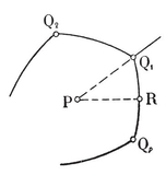
Secondly, if there is just one axis of p-fold rotation where p>2, this must be perpendicular to any digonal axes that may occur. Hence the group is either cyclic of order p or dihedral of order 2p.
Finally, if there are several axes of more than 2-fold rotation, let one of them be OP, so that there is a rotation through 2π/p about P. The group being finite, there is a least distance from P (on the sphere) at which we can find a point Q1 lying on another axis of more than 2-fold rotation, say q-fold rotation. Successive rotations through 2π/p about P transform Q1 into other centres of q-fold rotation, say Q2, . . . , Q*p, lying on a small circle within which P is the only centre of more than 2-fold rotation. (See Fig. 3.8A.) The product of rotations through 2π*/p and 2π/q about P and Q1 is the rotation through −2π/r about a point R such that the spherical triangle PQ1R has angles π/p, π/q, π/r.
We proceed to determine the position of R and the value of r. (We cannot yet say whether r is an integer.) Since the angle-sum of any spherical triangle is greater than π, we have
3·81
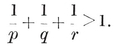
But p ≥ 3 and q ≥ 3. Hence r < 3, and consequently q > r. Thus the triangle PQ1R has a smaller angle at Q1 than at R, and the same inequality must hold for the respectively opposite sides. Hence R lies inside the small circle around P, and OR must be a digonal axis ; so the rotation through −2π/r about R, which transforms Q*p* into Q1, can only be a half-turn. Hence r = 2, and OR bisects the angle Q*pOQ1, i.e., R is the mid-point of the side Qp* Q1 of the spherical p-gon Q1 Q2 . . . Q*p. Successive rotations through 2π*/q about Q1 transform this p-gon (of angle 2π/q) into a set of q p-gons completely surrounding their common vertex Q1. Further rotations of the same kind lead to a number of p-gons fitting together to cover the whole sphere.
Thus the transforms of Q1 are the vertices of the regular polyhedron {p, q}, the transforms of P are the vertices of the reciprocal polyhedron {q, p}, and the transforms of R PQ1R was called P2 P0 P1 in § 2·5.)
From our construction we can be sure that the p-gonal and q-gonal axes through the vertices of {q, p} and {p, q P and Q1, if p = q ? No : that half-turn would combine with the rotation through 2π/p about P to give a rotation of period 4 about R, which is absurd.
3·9. Historical remarks. The kinematics of a rigid body (§ 3·1) was founded by Euler (1707-1783) and developed by Chasles, Rodrigues, Hamilton, and Donkin. In particular, 3·12 is commonly called “ Euler’s Theorem ”.
The theory of permutation groups (or “ substitution groups ”) was developed by Lagrange (1736-1813), Ruffini, Abel (1802-1829), Galois (1811-1832), Cauchy (1789-1857), and Jordan (whose famous Traité des Substitutions appeared in 1870). Lagrange proved that the order of a group is divisible by the order of any subgroup. Galois made such important contributions to the subject that he eventually became recognized as the real founder of group-theory ; yet his contemporaries scorned him, and he was murdered52 at the age of twenty. The notion of a self-conjugate subgroup is due to him, and it was he who first distributed the operations of a group into cosets (though the actual word “ co-set ” was coined in 1910 by G. A. Miller). The first precise definition of an abstract group was given in 1854 by Cayley (1).
In § 3·4 we considered the set of transforms of a single point by a group of congruent transformations. This idea occurs in a posthumous paper of Möbius (2). The rotation group of the regular polyhedron {p, q} was investigated in 1856 by Hamilton (1), who gave an abstract definition equivalent to
R*p* = S*q* = (RS)2 = 1.
The polyhedral groups also arose in the work of Schwarz and Klein, as groups of transformations of a complex variable. The first chapter of the latter’s Lectures on the Icosahedron (Klein 2) may well be read concurrently with §§ 3·5 and 3·6.
The compound polyhedra were thoroughly investigated by Hess in 1876.53 But the stella octangula {4, 3}[2] {3, 4} had already been discovered by Kepler (1, p. 271) and may almost be said to have been anticipated in Euclid XV, 1 and 2. It occurs in nature as a crystal-twin of tetrahedrite: The existence of the remaining compounds is a simple consequence of Kepler’s observation that a cube can be inscribed in a dodecahedron. It was Hess who first gave Cartesian coordinates for the vertices of all the regular and quasi-regular polyhedra,54 as in § 3·7.
A viendra en C.” Bravais’s proof occurs as part of the more complicated problem of enumerating the finite groups of congruent transformations, which includes the enumeration of the 32 geometrical crystal classes.55 This enumeration was first achieved in 1830, by Hessel (1), whose book remained unnoticed till 1891. The next step in the same direction was Sohncke’s enumeration of 65 infinite discrete groups of displacements. Finally, after Pierre Curie had drawn attention to the importance of the rotatory-reflection, the famous enumeration of 230 infinite discrete groups of congruent transformations was made independently by Fedorov in Russia (1885), Schoenflies in Germany (1891), and Barlow in England (1894).
[]
¶ CHAPTER IV
TESSELLATIONS AND HONEYCOMBS
THE limiting form of a p-gon, as p tends to infinity, is an infinite line broken into segments. We call this a degenerate polygon or apeirogon. Analogously, a plane filled with polygons (like a mosaic) may be regarded as a degenerate polyhedron, and so takes a natural place in this investigation. Conversely, we often find it useful to replace an ordinary polyhedron by the corresponding tessellation of a sphere. In § 4·5, for instance, we consider both plane and spherical tessellations at the same time. The analogous honeycombs (i.e., space filled with polyhedra) form a natural link between polyhedra in ordinary space and polytopes in four dimensions.
4·1. The three regular tessellations. A plane tessellation (or two-dimensional honeycomb) is an infinite set of polygons fitting together to cover the whole plane just once, so that every side of each polygon belongs also to one other polygon. It is thus a map with infinitely many faces (cf. § 1·4).
Let a finite portion of this map, bounded by edges, consist of N2 − 1 faces, N1 edges, and N0 vertices (including the peripheral edges and vertices). By regarding the whole exterior region as one further face, we obtain a “ finite ” map to which we can apply Euler’s Formula
N0 − N1 + N2 = 2.
This equation remains valid however much we extend the chosen finite portion by adding further faces. If the process of enlargement can be continued in such a way that the increasing numbers N0, N1 N2 tend to become proportional to definite numbers ν0, ν1, ν2, we conclude that
4·11
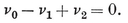
In particular, if all the faces are p-gons, and there are q
qν0 = 2ν1 = pν2,
and
4·12

or
(p − 2)(q − 2) = 4.
This result is not surprising, as it can be derived formally from 1·72 by making N1 tend to infinity. But that derivation could not be accepted as a proof; for there is no sequence of finite regular maps tending to an infinite regular map (like the polygons, {p}, which tend to the apeirogon, {∞}).
The solutions of 4·12, viz., {3, 6}, {4, 4}, {6, 3}, are exhibited (fragmentarily) in Fig. 4.1A. The second is merely “ squared paper “ ; the first is likewise available on printed sheets ; and the third is often seen as wire netting, or on the tiled floors of bathrooms. (The corresponding points in Fig. 2.3B are marked with black dots.)
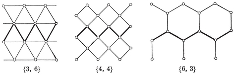
The criterion 4·12 can alternatively be obtained from easy metrical considerations, as follows. The definitions for vertex figure and regular are the same as in the case of polyhedra (§ 2·1). More simply, a tessellation is regular if its faces are regular and equal. A vertex of {p, q} is surrounded by q angles, each (1−2/p)π, which together amount to 2π*.* Hence 1−2/p=2/q.
Descartes’ Formula (in the form 2·51) is immediately verified for any tessellation, as δ=0 while No is infinite.
Since 6 is even, the edges of {3, 6} can be coherently indexed like those of the octahedron (page 51). The appropriate ratio in which to divide them is 2 : 1, but the result is merely a smaller {3, 6}.
4·2. The quasi-regular and. rhombic tessellations. If {3, 6} and {6, 3} are drawn on such a scale that their edges are in the ratio √3 : 1 (see 2·71), they can be superposed to form dual maps. In fact, their respective edges can bisect each other, as in Fig. 4.2A. By analogy with § 2·2, we then call them reciprocal tessellations, although there is no reciprocating sphere. The common mid-points of their edges are the vertices of the quasi-regular Fig. 4.2B. The crossing edges themselves are the diagonals of rhombs which form the reciprocal rhombic tessellation shown in Fig. 4.2C.
 its reciprocal are smaller {4, 4}’s (rotated through 45°). Thus the equation
4·21
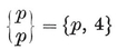
(cf. 2·31) holds when p=4 as well as when p p}’s and 2 {q}’s at each vertex.)
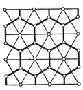
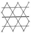
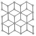
Two reciprocal {4, 4}’s together have the vertices of a smaller {4, 4}, and so can be regarded as forming a self-reciprocal “ compound tessellation ” {4, 4)[2]{4, 4}, analogous to the stella octangula (§ 3·6). Since alternate vertices of a {6, 3} of edge 1 belong to a {3, 6} of edge √3, there is another such compound, {6, 3)[2], consisting of two {3, 6}’s inscribed in a {6, 3} (Fig. 4.2D). The reciprocal of the {6, 3} is a third {3, 6} of edge √3, so we have altogether three {3, 6}’s of edge √3 inscribed in a {3, 6} of edge 1. Here (Fig. 4.2F) pairs of faces are concentric with the faces of a {6, 3}, so the appropriate symbol is
{3, 6}[3]2.
The reciprocals of these compounds are, of course, [2]{3, 6} and
2[3]
(Figs. 4.2E· and G). For the complete list of such compounds see Coxeter, Proceedings of the Royal Society, (A), 278 (1964), p. 148.
In virtue of 4·12, 2·33 yields h

FIG. 4.2D : {6, 3}[2{3, 6}]
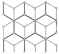
FIG. 4.2E : [2{6, 3}]
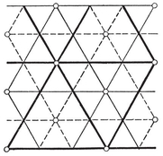
FIG. 4.2F: {3, 6}[3{3, 6}]2
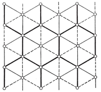
FIG. 4.2G: 2{3, 6}[3{6, 3}]
Fig. 4.2B, and the Petrie polygons of the regular tessellations are plane zigzags (emphasized in Fig. 4.1A).
According to 2·42 and 2·43, all the radii jR are infinite. This is natural, as any tessellation can be regarded as a “ degenerate ” polyhedron whose centre, O3, has receded to infinity. The same explanation applies to the manner in which 2·44 yields
φ = χ = ψ = 0.
Moreover, it is evidently correct to say that the dihedral angle is just π.
4·3. Rotation groups in two dimensions. The following statements can be verified without difficulty. The symmetry group of a regular tessellation is an infinite group of congruent transformations in the plane. It contains transformations of all four kinds : reflections, rotations, translations, and glide-reflections. (See page 36.) There is a subgroup of index 2 consisting of translations and rotations alone, these being the only displacements. We call this subgroup a rotation group even though it contains translations. (For these, after all, can be regarded as a limiting case of rotations.) The translations by themselves form a self-conjugate subgroup in either of the other groups. This translation group is a special case of the lattice group generated by two translations in distinct directions. The transforms of any point by such a group make a two-dimensional lattice, consisting of the vertices of a tessellation whose faces are equal parallelograms, all orientated the same way (unlike the rhombs of Fig. 4.2C, which are orientated three different ways). This notion is important in the theory of elliptic functions.
The enumeration of discrete groups of displacements in the plane is closely analogous to that of finite groups of rotations in space, as carried out in § 3·8. The conclusion is that there are eight such groups :
(i) the finite cyclic group generated by a rotation through 2π/p ;
(ii) the infinite cyclic group generated by a translation ;
(iii) the infinite dihedral group 56 generated by two half-turns (whose product is a translation) ;
(iv) the lattice group, generated by two translations ;
(v) the group generated by half-turns about three non-collinear points, i.e., the rotation group of a lattice ;
(vi) the rotation group of {3, 6}, or of {6, 3}, generated by a half-turn and a trigonal rotation ;
(vii) the rotation group of {4, 4}, generated by a half-turn and a tetragonal rotation, or by two tetragonal rotations;
(viii) the group generated by two trigonal rotations—a subgroup of (vi).
The last of these arises from the fact that the equation
4·31
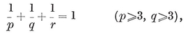
which replaces 3·81, does not imply r=2, but has the “extra ” solution p = q = r = 3.
One important fact which emerges from the above list is the “ crystallographic restriction ” :
4·32. If a discrete group of displacements in the plane has more than one centre of rotation, then the only rotations that can occur are *2-fold, 3-*fold, 4-fold, and 6-fold.
This theorem (which is closely related to Haüy’s crystallographic “Law of Rationality ”) can be proved directly, as follows.
Let P be a centre of p-fold rotation, and Q one of the nearest other centres of p-fold rotation. Let the rotation through 2π/p about Q transform P into P′, and let the same kind of rotation about P′ transform Q into Q′, as in Fig. 4.3A. It may happen that P and Q′ coincide ; then p=6. In all other cases we must have PQ′ ≥ PQ; therefore p ≤ 4. (This simple proof is due to Barlow.)
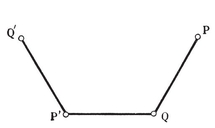
We have now reached a suitable place to introduce the important notion of a fundamental region. For any group of transformations of a plane (or of space), this means a region whose transforms just cover the plane (or space), without overlapping and without interstices. In other words, every point is equivalent (under the group) to some point of the region, but no two points of the region are equivalent unless both are on the boundary. Thus the eight groups described above have the following fundamental regions:
(i) an angular region (bounded by two rays) of angle 2π/p ;
(ii) an infinite strip (bounded by two parallel lines) ;
(iii) a half-strip (bounded by two parallel rays and a perpendicular segment) ;
(iv) a parallelogram (with translations along its sides) ;
(v) a parallelogram (with half-turns about the mid-points of its sides) ;
(vi) an equilateral triangle (with a hexagonal rotation about one vertex, and trigonal rotations about the other two) ;
(vii) a square (with tetragonal rotations about two opposite vertices, and half-turns about the other two) ;
(viii) a rhomb of angle *π/*3 (as in Fig. 4.2C).
4·4. Coordinates for the vertices. The vertices of a {4, 4} of unit edge may be described as the points whose rectangular Cartesian coordinates are integers.
x, y) for which x±y
 x, y) for which x and y are not both even. For, these are the mid-edge points of the {3, 6} of edge 2 for which x and y are both even. The vertices of the reciprocal rhombic tessellation are, of course, the same as those of {3, 6} ; it is the edges and faces that are different.
Returning to rectangular coordinates, let the point (x, y) represent the complex number z=x+yi. Then the vertices of {4, 4} represent the Gaussian integers (for which x and y are ordinary integers). The rotation group of {4, 4} is generated by the translation
z′ = z + 1
and the tetragonal rotation
z′ = iz*.*
Similarly, the rotation group of {3, 6} is generated by the same translation along with the hexagonal rotation

Hence the vertices of {3, 6} represent the algebraic integers u+vω (where u and v are ordinary integers).
4·5. Lines of symmetry. By projecting the edges of a polyhedron from its centre onto a concentric sphere, as in § 1·4, we obtain a set of arcs of great circles, forming a map. The theory of such maps is so closely analogous to that of plane tessellations that one is tempted to call them spherical tessellations. In the following treatment of lines of symmetry, we shall consider both kinds of tessellation simultaneously ; e.g., {4, 3} will not mean the cube, but the map of six equal regular spherical quadrangles covering a sphere.
Taking the sphere to be of unit radius we have, instead of a regular polyhedron {p, q} of edge 2l, a spherical tessellation {p, q} of edge 2φ, whose faces are spherical p-gons of angle 2π/q, as in § 3·8. The properties χ and ψ L
L π/h, whose faces are spherical p-gons and q-gons of circum-radii ψ and φ, respectively. The reciprocal is a spherical tessellation of edge χ, whose faces are spherical “ rhombs ” of angles 2π/p, 2π/q
If a plane (or solid) figure is symmetrical by reflection in a certain line (or plane) w, we call w a line of symmetry (or plane of symmetry). We saw in § 3·4 that the regular polygon {p} has p lines of symmetry. When p is odd, each joins a vertex to the mid-point of the opposite side. But when p
In Figs. 4.5A and B57 we have marks 0, 1, 2 at all the vertices, mid-points of edges, and centres of faces, of the regular tessellations {3, 3}, {3, 4}, {3, 5}, {3, 6}, and {4, 4}. (The corresponding figures for {4, 3}, {5, 3}, {6, 3} can be derived by interchanging the marks 0 and 2.) In other words, the points marked 0, 1, 2 are the vertices of the three related tessellations {p, q 2, and (01010101) to (01)4:
{3, 3} has 6 lines (010212) ;
{3, 4} has 6 lines (0212)2 and 3 lines (01)4;
{3, 5} has 15 lines (010212)2;
{3, 6} has ∞ lines (0212)∞ and ∞ lines (01)∞;
{4, 4} has ∞ lines (01)∞, ∞ lines (02)∞, and ∞ lines (12)∞.
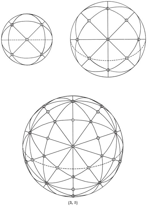
We have not mentioned the “improper” tessellations, where p or q = 2, because much of the following discussion would break down if applied to them. The discussion will lead us to a simple expression for the number of lines of symmetry. For a plane tessellation this number is, of course, infinite ; so let us restrict consideration to a proper spherical tessellation {p, q}.
The lines of symmetry divide the spherical surface into a tessellation of congruent triangles 012, like the triangle P0 P1 P2 described at the end of § 2·5. Since each point 1 is surrounded by four of the triangles, the total number of triangles is 4N1, where N1 is given by 1·72. Since each segment 01 or 02 or 12 belongs to two of the triangles, there are 2N1 segments of each type altogether. (The 2N1 segments 01 are just the halves of the N1 edges of {p, q 02. Thus the equator in which any equatorial polygon is inscribed (see page 18) contains h points 1 and crosses h segments 02.
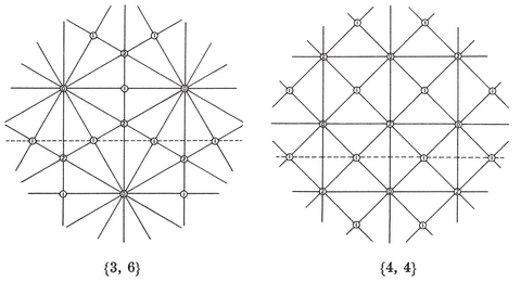
A line of symmetry is met by the 2N1/h equators in the following manner. Any two antipodal points 1 belong to two of the equators, and any two antipodal segments 02 are crossed by one of the equators.58 Since each point 1 belongs to two adjacent segments 01 or 12, it follows that the number of segments (or of marked points) on a line of symmetry of any type is equal to twice the number of equators, viz., 4N1/h.
An equator is met by the lines of symmetry in the following manner. Each point 1 lies on two lines of symmetry, and each segment 11 (i.e., each side of the equatorial polygon) is crossed by one line of symmetry. Since the equatorial polygon has h/2 pairs of opposite vertices and h/2 pairs of opposite sides, the total number of lines of symmetry is 3h/2.
Combining this result with 2·34, we may say that a regular solid with N1 p, 2} and the hosohedron {2, p}. A slightly more complicated expression that applies also to these insubstantial “ solids ” is
h − 1 + 2N1/h,
where h is given by 2·33.
4·6. Space filled with cubes. A three-dimensional honeycomb (or solid tessellation) is an infinite set of polyhedra fitting together to fill all space just once, so that every face of each polyhedron belongs to one other polyhedron. There are thus vertices Π0, edges Π1, faces Π2, and cells (or solid faces) Π3: in brief, j-dimensional elements Πj (j=0, 1, 2, 3). As in § 1·8, we let Njk (j≠k) denote the number of Πk’s that are incident with a single Π*j* ; e.g.,
4·61
For each Π2 or Π1, respectively, we have
4·62
A honeycomb is said to be regular if its cells are regular and equal. If these are {p, q}’s, and r of them surround an edge (so that N12=N13=r), then the honeycomb is denoted by {p, q, r}. The number r must be the same for every edge, as it necessitates a dihedral angle 2π/r for the cell. Moreover, Table I shows that the cube is the only regular polyhedron whose dihedral angle is a submultiple of 2π. Hence the only regular honeycomb is {4, 3, 4}, the ordinary space-filling of cubes, eight at each vertex.
This can alternatively be seen as follows. The mid-points of all the edges that emanate from a given vertex are the vertices of a polyhedron called the vertex figure of the honeycomb ; its faces are the vertex figures of the cells that surround the given vertex. (For instance, the vertex figure of {4, 3, 4} is an octahedron.) If the edges of the honeycomb are of length 2l, the vertex figure has a circum-sphere of radius l. If all the faces are {p}’s, the edges of the vertex figure (being vertex figures of {p}’s) are of length 2l cos π/p. Thus the vertex figure of a honeycomb {p, q, r} of edge 2l must be a {q, r} of edge 2l cos π/p, whose circum-radius is l. But (by Table I again) the only regular polyhedron whose edge and circum-radius have a ratio of the form 2 cos π/p is the octahedron, for which this ratio is √2=2 cos π/4. Hence {p, q, r} can only be {4, 3, 4}.
[image]{.image .placeholder original-image-src=“content/images/00114” original-image-title=“” width=“0in” height=“0in”}p, q, r} as the result of telescoping the respective symbols {p, q} and {q, r} for the cell and vertex figure.
[image]{.image .placeholder original-image-src=“content/images/00114” original-image-title=“” width=“0in” height=“0in”}[image]{.image .placeholder original-image-src=“content/images/00114” original-image-title=“” width=“0in” height=“0in”}π for their sum ; these can only be a tetrahedron and an octahedron, where the sum is π. Or we look at the possible vertex figures, admitting the cuboctahedron whose edge is equal to its circum-radius, and discarding the icosidodecahedron (for which the ratio of edge to circum-radius is 2 sin π/h=2 sin π/10=2 cos 2π/5). From either point of view, we conclude that there is only one quasi-regular honeycomb.59 Each vertex is surrounded by eight tetrahedra and six octahedra (corresponding to the triangles and squares of the cuboctahedron). All the faces are triangles ; each belongs to one {3, 3} and one {3, 4}. Thus an appropriate extension of the Schläfli symbol is

For the development of a general theory, it is an unhappy accident that only one honeycomb is regular, and only one quasi-regular. Of course, there are many with a slightly lower degree of regularity : “semi-regular”, let us say. For instance, 60 l and lateral edges l√2.
The relationship of these figures is very simply seen with the aid of rectangular Cartesian coordinates. All the points whose three coordinates are integers are the vertices of a {4, 3, 4} of edge 1. Those whose coordinates are all even belong to a {4, 3, 4} of edge 2. Those whose coordinates are all odd form another equal {4, 3, 4}. These two {4, 3, 4}’s of edge 2 are said to be reciprocal,
Let the points with integral coordinates (x, y, z) be marked 0, 1, 2, or 3 according to the number of odd coordinates, as in Fig. 4.7A. These points correspond to the elements Π0, Π1, Π2, Π3 of one of our two reciprocal {4, 3, 4}’s, and to the elements Π3, Π2, Π1, Π0 of the other. The points 1 (or 2 0 and 2 together (or 1 and 3
 sum.
sum.
 stella octangula).
 61 The in-spheres of its cells form the “ cubic close-packing ” or “ normal piling ” of spheres —a fact which is sometimes adduced as a reason for the resemblance between this particular space-filling and the honeycomb actually constructed by bees.
The planes of symmetry of {4, 3, 4} are its face-planes and the planes of symmetry of its cells. They are thus of three distinct types (containing points 0, 1, 2 ; 0, 1, 2, 3 ; and 1, 2, 3) and intersect in axes of symmetry of six types : tetragonal axes (01)∞ and (23)∞, trigonal axes (03)∞, and digonal axes (02)∞, (12)∞, (13)∞. These planes and lines form a honeycomb of congruent quadrirectangular tetrahedra 0123, whose edges 01, 12, 23 are mutually perpendicular.62 (See Fig. 4.7A.)
Such a tetrahedron is in some respects a more natural analogue for the right-angled triangle than is the trirectangular tetrahedron (where all the right angles occur at one vertex). Just as any plane polygon can be dissected into right-angled triangles, so any solid polyhedron can be dissected into quadrirectangular tetrahedra. A special feature of the characteristic tetrahedron 0123 is that the perpendicular edges 01, 12, 23 are all equal (so that the remaining edges are of lengths √2, √3, √2 ; in fact the edge ij i<j).
i<j).
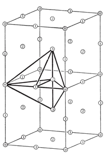
All the points 0, 2, 3 (without 1) form a honeycomb of trirectangular tetrahedra 0023, 0 and 2, but a larger specimen whose vertices are alternate points 0). This trirectangular tetrahedron 0023, whose edge 00 is of length 2, can be obtained by fusing two quadrirectangular tetrahedra 0123 which have a common face 123.
Finally, the points 0 and 3 together form a honeycomb of tetragonal disphenoids (or “ isosceles tetrahedra ”) 0033, each of which is obtained by fusing two trirectangular tetrahedra 0023 which have a common face 002. The opposite edges 00 and 33 are both of length 2, and the four edges 03 are all of length √3.
[image]
[image]{.image .placeholder original-image-src=“content/images/00114” original-image-title=“” width=“0in” height=“0in”}[image]{.image .placeholder original-image-src=“content/images/00114” original-image-title=“” width=“0in” height=“0in”}N3−1 cells, N2 faces, N1 edges, and N0Njk is understood to be summed over all the Π*j*’s, we have
[image]
[image]
N30 − N31 + N32 = 2,
N01 − N02 + N03 = 2.
Summing these expressions over all cells and all vertices, respectively, and subtracting, we obtain
N30N03N31N02N32N01) = 2N3 − 2N0.
N30N03N31N13N1221N20N02[image]{.image .placeholder original-image-src=“content/images/00114” original-image-title=“” width=“0in” height=“0in”}N32N01N23N10 = 2N2 − 2N1[image]{.image .placeholder original-image-src=“content/images/00114” original-image-title=“” width=“0in” height=“0in”}N2 − 2N1 = 2N3 − N0, or N0 − N1 + N2 − N3 = 0.63
If the chosen portion can be enlarged in such a way that the increasing numbers Nj tend to become proportional to definite numbers νj, we conclude that
[image]
[image]
For a portion of a regular[image]
ν*j* Njk = ν*k* Nkj
for the whole honeycomb. In particular, taking ν0 = 1, we have
[image]
Here N01, N02, and N03 are simply the numbers of vertices, edges, and faces of the vertex figure. Hence, for {4, 3, 4}, whose vertex figure is an octahedron, we have

In brief, ν*j* (1−1)3. (See Table II on page 296.)
[image]{.image .placeholder original-image-src=“content/images/00114” original-image-title=“” width=“0in” height=“0in”}Π*j*
[image]
1 − 6 + 8 − (2 + 1) = 0**.**
[image]{.image .placeholder original-image-src=“content/images/00114” original-image-title=“” width=“0in” height=“0in”} Plane tessellations were discussed by Kepler, who seems to have been the first to recognize them as analogues of polyhedra.64 But spherical tessellations, both regular and quasi-regular, were described by Abû’l Wafa (940-998).65 The notion of reciprocal[image]
[image]{.image .placeholder original-image-src=“content/images/00114” original-image-title=“” width=“0in” height=“0in”}66 enumerated by Pólya and Niggli in 1924.
[image]{.image .placeholder original-image-src=“content/images/00114” original-image-title=“” width=“0in” height=“0in”}3h/2 great circles, each decomposed by the rest into 4N1/h=h+2 arcs (altogether 6N1 arcs, the sides of 4N1 triangles), and that the “ equators ” consist of 2N1/h great circles, each decomposed by the rest into h arcs (altogether 2N1 arcs, the sides of N2 = 2N1/p {p}’s and N0=2N1/q {q}’s). The 3h/2 “ lines ” of symmetry intersect one another in 3h(3h − 2)/4 points, of which p(p − 1)/2 coincide at each of the N2 points 2, q(q − 1)/2 at each of the N0 points 0, while each of the N1 points 1 appears once. Hence
Since 4N1 = h(h[image]
[image]
(Steinberg 1). Since the sides of the 4N1 triangles 012 are arcs of the 3h/2 lines of symmetry, each described twice, we have
4N1(φ + χ + ψ) = 3h[image]
whence
[image]
in agreement with the observation of Hess67 and Brückner 68 that φ + χ + ψ is always commensurable with π.

The notion of reciprocal honeycombs seems to be due to Andreini (1), whose monograph is handsomely illustrated with stereoscopic photographs. The present treatment is intended as a preparation for the study of four-dimensional polytopes in Chapters VII and VIII.
[]
¶ CHAPTER V
THE KALEIDOSCOPE
THIS is an account of the discrete groups generated by reflections, including as special cases the symmetry groups of the regular polyhedra and of the regular and quasi-regular honeycombs. The analogous groups in higher space will be found in Chapter XI.
[image]{.image .placeholder original-image-src=“content/images/00114” original-image-title=“” width=“0in” height=“0in”} When an object is held in front of an ordinary mirror, two things are seen : the object and its image. If Alice could take us through the looking-glass, we would still see the same two things, for the image of the image is just the original object. In other words, a single reflection R generates a group of order two, whose operations are 1 and R. There are no further operations, since
[image]

and consequently R−1=R. Instead of a plane mirror in space, we can just as well use a line-mirror in a plane, or a point-mirror in a line. A point divides a line into two half-lines or rays, and serves as a mirror to reflect the one ray into the other.
But when an object is held between two parallel mirrors, there is theoretically no limit to the number of images ; for there are images of images, ad infinitum. The mirrors themselves have infinitely many images : virtual mirrors which appear to act like real mirrors. In other words, two parallel reflections, R1 and R2, generate an infinite group whose operations are
1, R1, R2, R1 R2, R2 R1, R1 R2 R1, R2 R1 R2, . . . .
As an abstract group, this is called the “ free product ” of two groups of order two; it has the generating relations R12=1, R22=1, or, briefly,
[image]
We can just as well regard the R’s as reflections in two parallel lines of a plane, or in any two points on a line. The two points and their images (the virtual mirrors) divide the line into infinitely many equal segments, which can be associated with the operations of the group, as follows. The segment terminated by the two given points (i.e., the region of possible objects) is associated with the identity, 1 ; and any other of the segments is associated with that operation which transforms the segment 1 into the other segment. (See Fig. 5.1A.)
Let any point and all its images (or transforms) be called a set of equivalent points. Then every point on the line is equivalent to some point of the segment 1 (including its end points), but no two distinct points of the segment are equivalent to each other. Thus the segment is a fundamental region for the group generated by R1 and R2. (See page 63.) Similarly, the group generated by R alone has a ray for its fundamental region, and the two complementary rays are associated with the two operations 1 and R.
Two intersecting mirrors form an ordinary kaleidoscope. This can be made very easily by joining two square, unframed mirrors with a strip of adhesive tape, so that the angle between them can be varied at will, and standing them on a table (with the taped edge vertical). Taking a section by a plane perpendicular to both mirrors (or considering the surface of the table-top alone), we reduce the kaleidoscope to its two-dimensional form, where we reflect in two intersecting lines. Since the images of any point (save the point where the lines meet) are distributed round a circle, the group is discrete 70 only if the angle between the mirrors is commensurable with π.
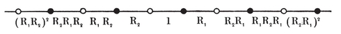
It will be sufficient to consider submultiples of π ; for if the angle is jπ/p, where j and p are co-prime, we can find a multiple of j/p which differs from 1/p by an integer, and hence a virtual mirror inclined at π/p[image]
Accordingly, we place an object between two mirrors inclined at π/p, and observe 2p images (including the object), one in each of the angular regions formed by the real and virtual mirrors. (The case when *p=*3 is shown in Fig. 5.1B.) Here the group is of order 2p, and its fundamental region is the angular region of magnitude π/p formed by the two rays that represent the mirrors. Each operation has two alternative expressions (e.g., R1 R2 R1 and R2 R1 R2 for the operation not named in Fig. 5.1B) according to which generator we use first. But these expressions are equal in virtue of the generating relations
[image]
We shall find it convenient to use the symbol [p] to denote this group of order 2p[image]{.image .placeholder original-image-src=“content/images/00114” original-image-title=“” width=“0in” height=“0in”}p = 1 imply R1=R2, and so reduce to R12=1 ; but the relation (R1 R2)∞ = 1 must be regarded as stating merely that the element R1 R2 is not periodic.)
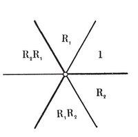
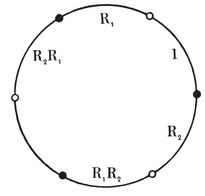
The manner in which [ ∞ ] arises as a limiting case of [p] is most clearly seen when we take the section of the mirrors by a circle with its centre at their point of intersection, and regard the R’s as reflections in points on this circle. Then the fundamental region is an arc, as in Fig. 5.1C. The transforms of one of the reflecting points (or of one end of the arc) are the vertices of a regular polygon {p}. (In Fig. 5.1C, this is a triangle.) Conversely, [p] is the complete symmetry group of {p}, i.e., [p] is the dihedral group of order 2p, as defined on page 46. Its cyclic subgroup of order p is generated by the rotation R1 R2.
When p[image]
R12 = 1, R22 = 1, R2 R1 = R1 R2.
Thus [2] is the direct product of two groups of order two (generated by the respective reflections, which now commute). The appropriate symbolism is
[image]
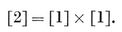
[image]{.image .placeholder original-image-src=“content/images/00114” original-image-title=“” width=“0in” height=“0in”} The group generated by reflections in any number of lines is equally well generated by reflections in these lines and all their transforms (the virtual mirrors). If the group is discrete, the whole set of lines effects a partition of the plane into a finite or infinite number of congruent convex regions, and the group is generated by reflections in the bounding lines of any one of the regions.
The reader will probably be willing to accept the statement that this is a fundamental region, especially if he has looked at three or four material mirrors standing vertically on a table, with a candle for object. It is obvious that every point of the plane is equivalent to some point in the initial region, but not obvious that two distinct points of this region cannot be equivalent. (In the elliptic plane, two such points can be equivalent.) However, we shall postpone the complete proof till § 5-3, where we discuss the general theory in three dimensions, from which this two-dimensional theory can be derived as a special case.
The internal angles of the region must be submultiples of π, as otherwise it would be subdivided by virtual mirrors. Thus the possible angles are π/2, π/3, . . ., none of them obtuse. This remark facilitates the actual enumeration of cases. In particular, it rules out the possibility that a region might have more than four sides.
A triangular region with angles π/p, π/q, π/r[image]{.image .placeholder original-image-src=“content/images/00114” original-image-title=“” width=“0in” height=“0in”}p q r) must be
(3 3 3) or (2 4 4) or (2 3 6)
(or a permutation of these numbers). We thus have an equilateral triangle, an isosceles right-angled triangle, and one half of an equilateral triangle (see Fig. 5.2A). The corresponding groups are denoted respectively by
[image]
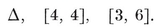
The two last are the complete symmetry groups of the regular tessellations (cf. Fig. 4.5A).
The other possible regions are : a half-plane, an angle, a strip, a half-strip, and a rectangle. The corresponding groups are
[1], [p], [ ∞ ], [ ∞ ] × [1], [ ∞ ] × [ ∞ ].
The last three are the groups that occur when we have mirrors in two opposite walls of an ordinary room, or in three walls, or in all four.
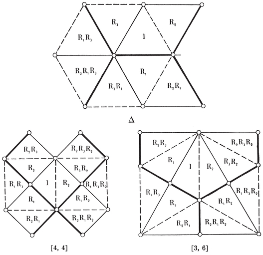
[image]{.image .placeholder original-image-src=“content/images/00114” original-image-title=“” width=“0in” height=“0in”} The group generated by reflections in any number of planes is equally well generated by reflections in these planes and all their transforms. If the group is discrete, the whole set of planes effects a partition of space into a finite or infinite number of congruent convex regions, and the group is generated by reflections in the bounding planes of any one of the regions. Let these bounding planes or walls be denoted by w1, w2, . . . , and let R*i* denote the reflection in w*i. The dihedral angle between two adjacent walls, wi* and W*j, is π/pij, where pij(=pji) is an integer greater than 1. The case when wi* and w*j* are parallel may be included by allowing p*ij* to be infinite.
The generating reflections evidently satisfy the relations
[image]
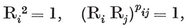
where the period of R*i* R*j* is specified for every edge of the region.
We proceed to prove that the region bounded by the w*’s is* a fundamental region for the group, and the relations [image]{.image .placeholder original-image-src=“content/images/00114” original-image-title=“” width=“0in” height=“0in”} suffice for an abstract definition. (This means that every true relation satisfied by the R’s is an algebraic consequence of these simple relations.)
[image]{.image .placeholder original-image-src=“content/images/00114” original-image-title=“” width=“0in” height=“0in”}s can be called, briefly, “region S”. Our only doubt is whether region S might coincide with region S’ for two distinct operations S and S′.
The rule for successively naming the various regions is as follows : we pass through the ith wall of region S into region R*i* S. This rule is justified by the fact that S transforms regions 1 and R*i, with their common wall wi, into regions S and Ri* S, with their common wall w*iswi, into oswiS. The reflection in the latter wall is Ri*s, which transforms oS 1 R2 R3 from region 1 in three stages : passing through the third wall of region 1 into region R3, then through the second wall of the latter into region R2 R3, and finally through the first wall of this into region R1 R2 R3. Thus the different names for a given region are given by different paths to it from region 1. (By a path we understand a continuous curve which avoids intersecting any edge.) Two such paths to the same region can be combined to make a closed path, which gives a new name, say
R*a* R*b* . . . R*k*,
for region 1 itself. If we can prove that the relations [image]{.image .placeholder original-image-src=“content/images/00114” original-image-title=“” width=“0in” height=“0in”} imply R*a* R*b* . . . R*k*=1, it will follow that the naming of regions is essentially unique, that region 1 is fundamental, and that the relations [image]{.image .placeholder original-image-src=“content/images/00114” original-image-title=“” width=“0in” height=“0in”} are sufficient.
For this purpose, we consider what happens to the expression R*a* R*b* . . . R*k* when the closed path is gradually shrunk (like an elastic band) until it lies wholly within region 1. Whenever the path goes from one region into another and then immediately returns, this detour may be eliminated by cancelling a repeated R*i* in the expression, in accordance with the relation R*i2=1. The only other kind of change that can occur during the shrinking process is when the path momentarily crosses an edge (common to 2pij* regions). This change will replace R*i* R*j* R*i* … by R*j* R*i* R*j* .
.
The shrinkage of the path thus corresponds to an algebraic reduction of the expression R*a* R*b* … R*k* by means of the relations [image]{.image .placeholder original-image-src=“content/images/00114” original-image-title=“” width=“0in” height=“0in”} The possibility of shrinking the path right down to a point (or to a small circuit within region 1) is a consequence of the topological fact that Euclidean space is simply-connected. It follows that R*a* R*b* . . . R*k*=1, as desired.
Incidentally, every reflection that occurs in the group is conjugate to one of the generating reflections. For, if it is the reflection in the ith wall of region S, it is expressible as R*i*s.
[image]{.image .placeholder original-image-src=“content/images/00114” original-image-title=“” width=“0in” height=“0in”}[image]{.image .placeholder original-image-src=“content/images/00114” original-image-title=“” width=“0in” height=“0in”}p]). In all other cases the fundamental region is a spherical triangle. For, since the angle-sum of a spherical n-gon is greater than that of a plane n-gon, namely (n−2)π, at least one of the angles must be greater than (n−2)π/n ; so for n≥4 at least one angle must be obtuse.
The enumeration of groups generated by reflections in concurrent planes thus reduces to the enumeration of spherical triangles with angles π/p, π/q, π/r[image]{.image .placeholder original-image-src=“content/images/00114” original-image-title=“” width=“0in” height=“0in”}p q r) to be
(2 2 p), (2 3 3), (2 3 4), (2 3 5).
(The last three are illustrated in Fig. 4.5A.) The respective groups are denoted by
[image]
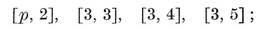
for, as we shall soon see, they are the complete symmetry groups of the dihedron, tetrahedron, octahedron (or cube), and icosahedron (or dodecahedron). To distinguish them from the rotation groups, these are known as the extended polyhedral groups.71
The fundamental region for [p, 2] is bounded by two meridians and the equator. Thus its kaleidoscope is formed by two (hinged) vertical mirrors standing on a horizontal mirror. Since the first two reflections both commute with the third, this group is a direct product :
[image]
The connection with the dihedron is explained on page 46.
[image]
[2, 2] = [1] × [1] × [1].
This is the group generated by three mutually commutative reflections (i.e., by three perpendicular mirrors).
The fundamental region for [p, q] (which is the same as [q, p]) is a triangle with angles π/p, π/q, π/2, whose area (if drawn on a sphere of unit radius) is
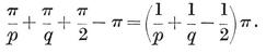
The order of [p, q] is the number of such triangles that will just cover the sphere (of area 4π), viz.,
[image]
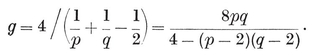
[image]{.image .placeholder original-image-src=“content/images/00114” original-image-title=“” width=“0in” height=“0in”}p, q[image]{.image .placeholder original-image-src=“content/images/00114” original-image-title=“” width=“0in” height=“0in”}p, q] are symmetry operations of {p, q[image]{.image .placeholder original-image-src=“content/images/00114” original-image-title=“” width=“0in” height=“0in”}p, q] is the complete symmetry group of {p, q}.
Each of the three “ trihedral kaleidoscopes ” is formed by three mirrors (preferably of polished metal) cut in the shape of sectors of a circle (of as large radius as is convenient, say 2 feet). The angles of these sectors are, of course, φ, χ, ψ. (See Table I on page 293.) The curved edges of the mirrors form the triangle P0 P1 P2[image]{.image .placeholder original-image-src=“content/images/00114” original-image-title=“” width=“0in” height=“0in”}Fig. 4.5A. An object placed at the vertex P0 (where 2q triangles meet) has images at all the points 0, viz., the vertices of {p, q}. Similarly an object at P1 or P2 (where 4 or 2p q, p}, respectively.
When {p, q} is a cube, so that the angle at P2 is π/4, the triangle P0 P1 P2 can be fused with its image in P1 P2 to form a right-angled triangle P0 P0′ P2 (Fig. 5.4A) which is the fundamental region for [3, 3]. The reflections in the sides of this larger triangle transform P0 and P0′ into the vertices of two reciprocal tetrahedra. Thus the stella octangula arises from the fact that the fundamental region for [3, 4] is one half of the fundamental region for [3, 3], which shows that the group [3, 4] contains [3, 3] as a subgroup of index two. Similarly, the infinite group [3, 6] contains Δ as a subgroup of index two. (See Figs. 4.2A[image]
[image]{.image .placeholder original-image-src=“content/images/00114” original-image-title=“” width=“0in” height=“0in”} We have completed the enumeration of groups generated by one, two, or three reflections. The groups generated by four or more reflections will be treated by more powerful methods in Chapter XI. It will then be seen that the following list is exhaustive.
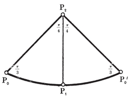
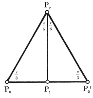
We may take one horizontal mirror with three or four vertical mirrors standing on it. Then the fundamental region is an infinitely tall prism, and the groups are the direct products
Δ × [1], [4, 4] × [1], [3, 6] × [1], [ ∞ ] × [ ∞ ] × [1].
(The last is the group that occurs when we have mirrors in all four walls of a room, and in the ceiling as well.)
Or we may take two horizontal mirrors (the upper facing downward) with two or three or four vertical mirrors between them. Then the fundamental region is an infinite wedge, or a triangular prism of three possible kinds, or a rectangular parallelepiped, and the groups are the direct products
[p] × [ ∞ ], Δ × [ ∞ ], [4, 4] × [ ∞ ], [3, 6] × [ ∞ ], [ ∞ ] × [ ∞ ] × [ ∞ ].
When p=2, the first of these splits further into [1] × [1] × [ ∞].
Finally, we may reflect in all four faces of a tetrahedron (provided the six dihedral angles are submultiples of π). The fundamental region may be the quadrirectangular tetrahedron 0123[image]{.image .placeholder original-image-src=“content/images/00114” original-image-title=“” width=“0in” height=“0in”}0023, or the tetragonal disphenoid 0033 ; and the groups are denoted by
[image]
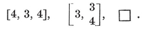

[image]{.image .placeholder original-image-src=“content/images/00114” original-image-title=“” width=“0in” height=“0in”} The various possible fundamental regions are very conveniently classified by associating them with certain graphs[image]{.image .placeholder original-image-src=“content/images/00114” original-image-title=“” width=“0in” height=“0in”}nodes of the graph represent the walls of the fundamental region (or the mirrors of the kaleidoscope, or the generating reflections), and two nodes are joined by a branch whenever the corresponding walls (or mirrors) are not perpendicular. Moreover, we mark the branches with numbers pij to indicate the angles π/pij (pij ≥ 3). Owing to its frequent occurrence, the mark 3 will usually be omitted (and left to be understood). Thus the fundamental region for [p] is denoted by

according as p=1 or 2 or 3 or more (including p = ∞ ).
The case when p[image]

representing the half-strip, rectangle, infinite wedge, infinitely tall prism on a rectangle, and rectangular parallelepiped, which are the fundamental regions for
[∞]×[1], [∞]×[∞], [p]×[∞], [∞]×[∞]×[1], [∞]×[∞]×[∞].
The reader can easily draw the graphs for the other prismatic regions in terms of the graphs
[image]
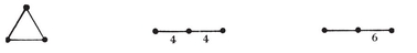
[image]

[image]
[image]
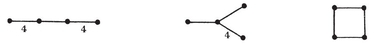
The convenience of this representation is seen in the following theorem :
[image]{.image .placeholder original-image-src=“content/images/00114” original-image-title=“” width=“0in” height=“0in”}. In the case of a connected graph without any even marks (e.g., if no branches are marked), all the reflections in the group are conjugate to one another.
To prove this, let R*i* and R*j* be two reflections represented by the nodes that terminate a branch with pij=2m+1 (e.g., an unmarked branch if m=1). Since (R*i* R*j*)2*m*+1 =1, we have
Thus R*i* and R*j* are conjugate. But the relation “ conjugate ” is. transitive, so the same conclusion holds if the ith and j[image]{.image .placeholder original-image-src=“content/images/00114” original-image-title=“” width=“0in” height=“0in”}all the reflections are conjugate.
For instance, the fifteen reflections in [3, 5] are all conjugate. More generally,
[image]{.image .placeholder original-image-src=“content/images/00114” original-image-title=“” width=“0in” height=“0in”} If we delete every branch that has an even mark (leaving its two terminal nodes intact), the resulting graph consists of a number of pieces equal to the number of classes of conjugate reflections in the group.
To prove this, consider what happens geometrically when two generators R*i* and R*j* are conjugate. It means that the ith wall of one region coincides with the jth wall of another, i.e., that the ith face of the former occurs in the same plane as the jth face of the latter. These two faces can be connected by a sequence of consecutively adjacent faces in the same plane. If two such adjacent faces are the ath of one region and the bth of another, the period of the product R*a* R*b* must be odd. (For, if a≠b, the two faces belong to a “ pencil ” of faces, pab of each kind, radiating from their common side. If a=b, the product is the identity, and the two faces may, for the present purpose, be considered as one.) Such a sequence of faces corresponds to a chain of odd-marked (or unmarked) branches connecting the ith and j[image]
[image]{.image .placeholder original-image-src=“content/images/00114” original-image-title=“” width=“0in” height=“0in”}p, q} has lines of symmetry of 1 or 2 or 3 types according as the symbol {p, q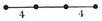
[image]{.image .placeholder original-image-src=“content/images/00114” original-image-title=“” width=“0in” height=“0in”} Wythoff’s construction π/p, and the second and third at π/q, while the first and third (not being directly joined by a branch) are perpendicular. These nodes can equally well be regarded as representing the respectively opposite vertices : one where the angle is π/q, one where it is π/2, and one where it is π/p. By drawing a ring around one of the nodes, we obtain a convenient symbol for the tessellation or polyhedron whose vertices are all the transforms of the corresponding vertex of the fundamental region, i.e., all the points 0 or 1 or 2 in Fig. 4.5A. Thus the modified graphs
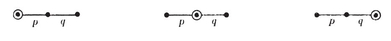
which can just as well be drawn as
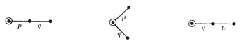
represent the respective tessellations (or polyhedra)
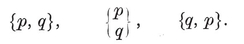
In fact, the Schläfli symbols may be regarded as abbreviations for the modified graphs.
 p
p
[image]{.image .placeholder original-image-src=“content/images/00114” original-image-title=“” width=“0in” height=“0in”}Fig. 4.7A) :
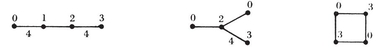
By drawing a ring around one of the nodes, we obtain a symbol for the honeycomb whose vertices are all the transforms of the corresponding vertex of the fundamental region. Thus the modified graph
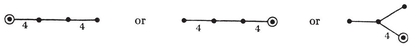
represents the regular honeycomb {4, 3, 4} ; similarly


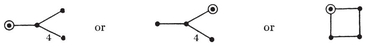

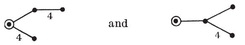
It is important to notice that the graphs for the polyhedra and honeycombs automatically contain the graphs for the various faces and cells.
[image]{.image .placeholder original-image-src=“content/images/00114” original-image-title=“” width=“0in” height=“0in”} In the fourth century A.D., Pappus observed that an icosahedron and a dodecahedron can both be inscribed in the same sphere in such a manner that the twelve vertices of the former lie by threes on four parallel circles, while the twenty vertices of the latter lie by fives on the same four circles. What is the general theory underlying this observation ?
In the trihedral kaleidoscope which illustrates the group [p, q] of order g[image]{.image .placeholder original-image-src=“content/images/00114” original-image-title=“” width=“0in” height=“0in”}g images, including the object itself. When the object, which we take to be a point, is moved towards a vertex P0 or P1 or P2 of the fundamental region (or towards the line of intersection of two of the three mirrors), the images approach one another in sets of 2q or 4 or 2p, at all the points 0 or 1 or 2. This shows clearly that the numbers of elements of {p, q} are
[image]
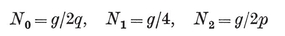
[image]
For any discrete group of congruent transformations, and any two points P and Q, we can prove that the distances from P to all the transforms of Q are equal (in some order) to the distances from Q to all the transforms of P. In fact, if S is any congruent transformation, the point-pair P, QSQ, from which it can be derived by applying S. Letting S denote each operation of the group in turn, we see that the various positions of QSP.
In particular, if the group is [p, q], and P, Q are P2, P0, then the transforms of Q coincide in sets of 2q at the vertices of {p, q}, while those of P coincide in sets of 2p at the vertices of {q, p} ; and we deduce that the distribution of vertices of {p, q} according to their distances from a vertex of the reciprocal {q, p} agrees with the distribution of vertices of {q, p} according to their distances from a vertex of its reciprocal {p, q}. In other words, if we distribute the vertices of {p, q} in circles, according to their various distances from the centre of one face, and then do the same for {q, p}, we will find that the two systems of circles are similar, and that the numbers of vertices occurring on corresponding circles are proportional (in the ratio p : q).
For instance, the twelve vertices of {3, 5} lie by threes on four circles in parallel planes, and the twenty vertices of {5, 3} lie by fives on four circles in parallel planes ; these can be taken to be the same four planes, provided the position and size of the two polyhedra are so adjusted that the planes of two opposite faces are the same for both. (This is a case where two polyhedra of reciprocal kinds are considered together without being in their actually reciprocal positions.)
The corresponding result for {3, 4} and {4, 3}, where two opposite faces account for all[image]{.image .placeholder original-image-src=“content/images/00114” original-image-title=“” width=“0in” height=“0in”}concentric circles, is again very simple, as the two tessellations can be so placed that the vertices of the former are alternate vertices of the latter (see Fig. 4.2D).
More complicated results of the same nature can be obtained by taking P to be P1, while Q is still P0. We then compare the distribution of vertices of {p, q}, q} ; e.g., the vertices of the dodecahedron, distributed in sets
2 + 4 + 2 + 4 + 2 + 4 + 2,
can lie in the same seven planes as the vertices of the icosidodecahedron, distributed in sets
3 + 6 + 3 + 6 + 3 + 6 + 3.
Again, we may apply the same theory to the group [4, 3, 4], taking Q to be a vertex of {4, 3, 4}, while P is (say) the centre of a square face. We then find that the vertices of {4, 3, 4}, distributed into sets
4 + 8 + 8 + 16 + 12 + 8 + 24 + …

12 + 24 + 24 + 48 + 36 + 24 + 72 + …
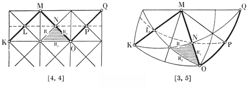
[image]{.image .placeholder original-image-src=“content/images/00114” original-image-title=“” width=“0in” height=“0in”}. Let R1, R2, R3 denote the reflections in the sides P1 P2, P2 P0, P0 P1 of the fundamental region for the group [p, q], where p and q are greater than 2. (It would perhaps have been more natural to call them R0, R1, R2.) To avoid confusing suffixes, let P0 and P1 be re-named O and N. The group transforms these into further points K, L, M, P, Q, as in Fig. 5.9A. In fact, R1 reflects O into M, R2 R1 rotates MN to KL, and R2 R3 rotates MN to QP. Now, KMOQ is part of a Petrie polygon for {p, q[image]{.image .placeholder original-image-src=“content/images/00114” original-image-title=“” width=“0in” height=“0in”}LNP R1 R2 R3 transforms KLMNO into MNOPQ ; i.e., it takes us one step along the Petrie polygon, and one step along the equatorial polygon. It thus consists of the translation or rotation that transforms LN into NP, combined with the reflection in LNP[image]{.image .placeholder original-image-src=“content/images/00114” original-image-title=“” width=“0in” height=“0in”}h[image]{.image .placeholder original-image-src=“content/images/00114” original-image-title=“” width=“0in” height=“0in”}the operation R1 R2 R3 is of period h.
[image]
[image]

Since g is always even, so also is h.
When [p, q] is finite, R1 R2 R3 is a rotatory-reflection involving rotation through 2π/h LNP ; and this possibility is excluded by our assumption that p and q are greater than 2. Hence the central inversion belongs to the group [p, q] (p>2, q>2) if and only ifis odd, and then it is expressible as

The first part of this theorem provides an arithmetical explanation for the fact that {3, 3} is the only one of the Platonic solids whose vertices do not occur in antipodal pairs.
Having observed the connection between the Petrie polygon for {p, q} and the operation R1 R2 R3 of [p, q], we naturally ask what kind of skew polygon is analogously related to the operation R1 R2 R3 R4 of [4, 3, 4]. Since R1 R2 R3 R4 is a screw-displacement, this will certainly be a helical polygon (see page 45). If its sides are edges of {4, 3, 4}, we shall feel justified in calling it a generalized Petrie polygon for that regular honeycomb.
Consider the helical polygon KLMNOP … (Fig. 5.9B) which is defined by the property that any three consecutive sides, but no four, belong to a Petrie polygon of a cell (i.e., of a cube). This will serve our purpose, provided we define the generating reflections as follows : R1 is the reflection in the perpendicular bisector of NO, and R2, R3, R4 are the reflections in the respective planes LMO, LNO, MNO. For these four planes form a suitable quadrirectangular tetrahedron ; and we have

whence R1 R2 R3 R4 transforms L into M, M into N, and N into O.
[image]{.image .placeholder original-image-src=“content/images/00114” original-image-title=“” width=“0in” height=“0in”}[image]
[image]{.image .placeholder original-image-src=“content/images/00114” original-image-title=“” width=“0in” height=“0in”}72 As a means for constructing regular and semiregular figures, its importance is more clearly seen in its extension to four dimensions, which Wythoff considered.73[image]
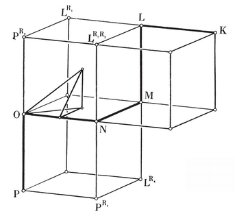
[image]{.image .placeholder original-image-src=“content/images/00114” original-image-title=“” width=“0in” height=“0in”}74
[image]
[]
¶ CHAPTER VI
STAR-POLYHEDRA
THIS chapter is mainly concerned with the four Kepler-Poinsot polyhedra (which are the first four figures in Plate III, facing page 49). Having agreed that these are polyhedra (according to a slightly modified definition), we cannot deny that they are regular.[image]
[image]{.image .placeholder original-image-src=“content/images/00114” original-image-title=“” width=“0in” height=“0in”} Star-polygons. Let S be a rotation through angle 2π/p, and let A0 be any point not on the axis of S. Then the points
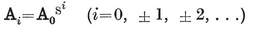
are the vertices of a regular polygon {p}, whose sides are the segments A0 A1, A1 A2, A2 A3, . . . (cf. page 45). When p[image]{.image .placeholder original-image-src=“content/images/00114” original-image-title=“” width=“0in” height=“0in”}p being integral; it is merely necessary that the period of S be finite, i.e., that p be rational. We shall still stipulate that p≥2, since a positive rotation through an angle greater than π is the same as a negative rotation through an angle less than π. Some instances are exhibited in Fig. 6.1A.
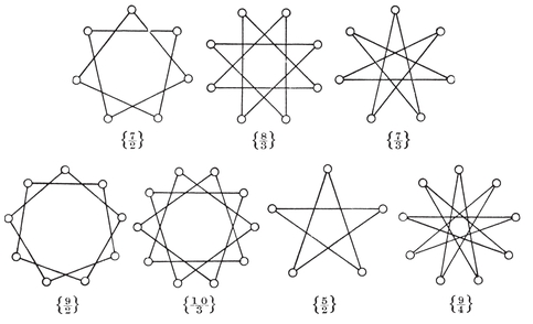
When the rational number pp and d*p. Thus p=np/dp, where np* and d*p* are co-prime integers. (When p is itself an integer, so that the polygon is convex, we naturally write n*p=p, dp=1.) The regular polygon {p} is traced out by a moving point which continuously describes equal chords of a fixed circle and returns to its original position after describing np* chords and making d*p* revolutions about the centre. Thus there are n*p* vertices and n*p* sides :
N0 = N1 = np.
When d*p>1, the sides of the “ star-polygon ” intersect in certain extraneous points, which are not included among the vertices. The digon, {2}, is to be considered as having two coincident sides. The number of different regular N-gons (N φ(N) is Euler’s function, the number of numbers less than N and co-prime to it.75 (N=np, to which both dp* and n*p−dp* are co-prime.)
The number d*p* is called the density of {p}, as it is the number of sides that will be pierced by a ray drawn from the centre in a general direction. (It is a happy accident that both words “ density ” and “ denominator ” begin with “ d.”)
The interior angle of {p[image]{.image .placeholder original-image-src=“content/images/00114” original-image-title=“” width=“0in” height=“0in”}p exterior angles is 2d*pπ*[image]{.image .placeholder original-image-src=“content/images/00114” original-image-title=“” width=“0in” height=“0in”}2l cos π/pτ-1l. (Cf. the vertex figure of {5}, which is of length τl[image]
S = 2n*pl*.
The area is still
[image]
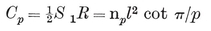
[image]{.image .placeholder original-image-src=“content/images/00114” original-image-title=“” width=“0in” height=“0in”}t times over the portions that are enclosed t times by the sides, for all values of t from 1 to d*p*.
The reciprocal of a {p} is evidently another {p}. If we choose for radius of reciprocation the geometric mean of 0R and 1R, the two reciprocal {p}’s will be equal ; when d*p* is even, this makes them actually coincide. The simplest of such completely self-reciprocal polygons is the pentagram,
The general regular polygon {p} can be derived from the convex polygon {n*p} by either of two reciprocal processes : stellating and faceting. In the former process, we retain the positions of the sides of {np}, and produce them at both ends, all to the same extent, until they meet to form new vertices. In the latter, we retain the vertices of {np} and insert a fresh set of sides, so that each new side subtends the same central angle as dp* old sides.
The same two processes also yield the regular compound polygons
{kn*p}[k{p}]{knp*},
such as the Jewish symbol {6}[2{3}]{6} which consists of two equal triangles in reciprocal positions.
[image]{.image .placeholder original-image-src=“content/images/00114” original-image-title=“” width=“0in” height=“0in”}[image]{.image .placeholder original-image-src=“content/images/00114” original-image-title=“” width=“0in” height=“0in”}small stellated dodecahedrongreat stellated dodecahedrongreat dodecahedrongreat icosahedronFig. 6.2A and Plate III, Figs. 1, 3, 2, 4.) We can construct these “Kepler-Poinsot polyhedra ” by stellating or faceting the ordinary dodecahedron and icosahedron.
In order to stellate a polyhedron, we have to extend its faces symmetrically until they again form a polyhedron. To investigate all possibilities, we consider the set of lines in which the plane of a particular face would be cut by all the other faces (sufficiently extended), and try to select regular polygons bounded by sets of these lines. For the tetrahedron or the cube, the only lines are the sides of the face itself. (The opposite face of the cube yields no line of intersection.) In the case of the octahedron, the faces opposite to those which immediately surround the particular face 111 meet the plane in a larger triangle 222 (Fig. 6.2B) whose sides 22 are bisected by the points 1. The eight large triangles so derived from all the faces form the stella octangula {4, 3}[2{3, 3}]{3, 4}. (Plate III, Fig. 5.)
Let us now stellate the dodecahedron {5, 3}, of which one face 11111 is shown in Fig. 6.2C.76 By stellating this pentagon we obtain the pentagram 2222222222Fig. 6.2C account for all the other faces of {5, 3}, the twelfth face being parallel to 11111.
To make sure that these stellations are single polyhedra, not compounds like the stella octangula,
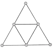
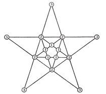
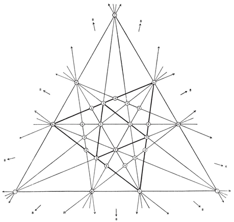
77 The eighteen lines of Fig. 6.2D are the intersections of the plane of the face 111 of {3, 5} with the planes of all the other faces save the opposite one. Their tangential barycentric coordinates, referred to the triangle 111, are the permutations of
(1, 0, 0), (τ, 1, 0), (τ, 1, τ−1), (1, 1, τ−1).
They form six concentric equilateral triangles, 111, 333, 3*′3′3′, 666, 6′6′6′, 777, each of which leads to a set of twenty when we apply the rotations of the icosahedral group. The twenty triangles 333 have no common sides, but when taken along with the twenty triangles 3′3′3′* they form the compound of five octahedra, [5{3, 4}]2{3, 5}. (See page 49.) The twenty triangles 666, and the twenty triangles 6*′6′6′*, are the faces of the two compounds of five tetrahedra
{5, 3}[5]{3, 5},
which are enantiomorphous and reciprocal, and which together form the compound of ten tetrahedra, 2{5, 3}[10
Having now constructed all the four Kepler-Poinsot polyhedra, we can record their properties Nj, as in Table I (page 292). We observe that N1pentagonal polyhedra [image]
[image]{.image .placeholder original-image-src=“content/images/00114” original-image-title=“” width=“0in” height=“0in”}. Faceting the Platonic solids. The above method is quite perspicuous when one has models to compare with the diagrams; but it would not be of much use to an inhabitant of Flatland.78 The reciprocal method of “ faceting,” however, lends itself more naturally to systematic treatment.
It is sometimes helpful to employ the following terminology. The core of a star-polyhedron or compound is the largest convex solid that can be drawn inside it, and the case is the smallest convex solid that can contain it ; e.g., the stella octangula has an octahedron for its core and a cube for its case, while the great icosahedron has an icosahedron for its core and another icosahedron for its case. The compound or star-polyhedron may be constructed either by stellating its core (which has the same face-planes) or by faceting its case (which has the same vertices). Thus stellating involves the addition of solid pieces, while faceting involves the removal of solid pieces.
For the systematic treatment of faceting, we first distribute the vertices of a Platonic solid Π (the “ case ”) in sets, according to their distances from a single vertex, O.[image]{.image .placeholder original-image-src=“content/images/00114” original-image-title=“” width=“0in” height=“0in”}ν vertices at distance a from O include the vertices of a {q} of side a, then each side of this {q} forms with O an equilateral triangle, and we have a {3, q} inscribed in Π. More generally, if the ν vertices at distance a include the vertices of a {q} of side b, where
b/a = 2 cos π/p
(for some rational value of p), and if a {p} of side a is known to occur among the vertices of Π, then we have a {p,q} inscribed in Π.
If ν=n*q*, so that the vertices of {q} are the only vertices of Π distant a from O, then either we find a single polyhedron {p, q} with the same vertices as Π, or (if {p, q} has fewer vertices than Π) we find several such polyhedra forming a vertex-regular compound
Π[d{p, q}],
where Π has d times as many vertices as {p, q}. On the other hand, if ν>n*q*, the possibility of a single polyhedron is ruled out. If the vertices of Π distant a from 0 include the vertices of c {q}’s (c≥1), we find a compound
cΠ[d{p, q}],
such that Π has d/c times as many vertices as {p, q}. Then, if d/c is an integer, say d′, it may be possible to pick out d′ of the d {p, q}′s so as to form Π[d′{p, q[image]
To carry out the required distribution of vertices of Π, we observe that the first set (after the point O itself) is at distance 2l, and belongs to a section similar to the vertex figure. If Π is the tetrahedron or the octahedron, the distribution is then complete (apart from the single opposite vertex of the octahedron). Otherwise, there is another set, antipodal to the first, at distance 2 1R. If Π is the cube or the icosahedron, the distribution is again complete. There remain for consideration two sets of six vertices of the dodecahedron. Using the coordinates 3·76 for a dodecahedron of edge 2τ−1, we find that the plane x + y + z = 1 contains the six vertices (0, −τ−1, τ), (1, − 1, 1), (τ, 0, −τ−1), (1, 1, −1), (−τ−1, τ, 0), (−1, 1, 1), which we are inclined to dismiss as an irregular hexagon, until we notice that they form two crossed triangles of side 2√2. These vertices are distant 2 from (1, 1, 1), and by reversing signs we find another such set distant 2√2.
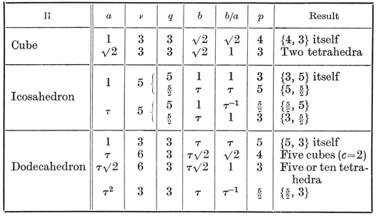
The only case where the location of {p} is not obvious is in the last line of the table. Alternate vertices of the dodecahedron’s Petrie polygon form a pentagon of side τ, which has the same vertices as the desired pentagram of side τ2. In Fig. 3.6E (where the peripheral decagon is the projection of a Petrie polygon), the pentagon is 12 23 34 45 51, and the pentagram is 12 34 51 23 45.
6·4. The general regular polyhedron. Most of the properties of {p, q}, as described in Chapter II, hold with but slight modifications when p or q Fig. 6.4A, the point seen in the middle is really at the bottom of a pit (bounded by three rhombs, which are parts of three large pentagons). Similarly, the small pentagon in the middle of Fig. 6.4B
 p, q} and {q, p}. In Fig. 6.4C, parts of three rhombs have been made transparent to reveal one of the twelve internal vertices (whence the broken lines radiate). At the middle of Fig. 6.4D
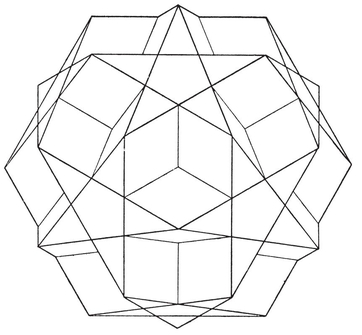

(12 pentagrams, 12 pentagons)

(12 pentagrams, 20 triangles)
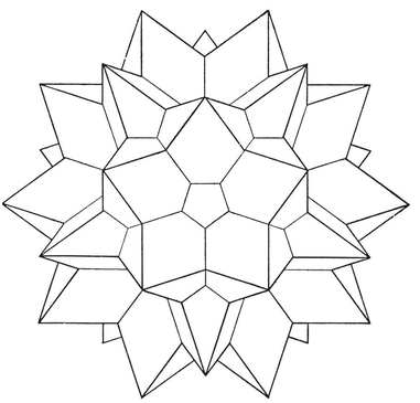
The Petrie polygon of {p, q h}, where h is given by 2·33. The rational number h is not necessarily an integer, so the number of sides of the Petrie polygon is the numerator, n*h, and the total number of Petrie polygons (or of equatorial polygons) is 2N*1/n*h*. But two equatorial polygons may intersect at other points than vertices, so 2·34 is no longer valid. Actually hN1 = 30 in each case, so the number of such polygons is 10 for the first two polyhedra, and 6 for the last two. (Figs. 6.2A and 6·4A, B are analogous to Figs. 2.6A and 2·3A.)
Formulae 2·41—2·45 continue to hold, provided we interpret Cp as in 6·11. Analogously, the volume is still given by 2·46, provided we define it as the sum of the volumes of the pyramids which join the centre to the faces. This means that, in stating the volume of a star-polyhedron, we count t times over the portions that are enclosed t times by the faces, enclosure by the pentagonal core of a pentagram counting twice. The maximum value of t, which occurs at the centre (and throughout the core of the polyhedron), is called the density of {p, q}, and is denoted by d*p*, *q*. In other words, the density is the number of intersections the faces make with a ray drawn from the centre in a general direction (counting two intersections for penetrating the core of a pentagram).
In order to obtain a formula for d*p*, *q*, we compute the number of times the surface of the concentric unit sphere is covered when we make a radial projection of the faces, as in § 2·5. Each face projects into a spherical {p} of angle 2π/q, which can be divided into n*p* isosceles triangles by joining its centre to its vertices. There are two such triangles for every edge of {p, q}, and each has spherical excess
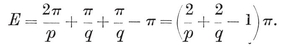
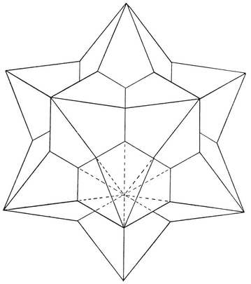
Small stellated triacontahedron
(30 rhombs)
Great stellated triacontahedron
(30 rhombs)
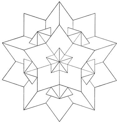
The multiply-covered sphere has area 4πd*p*, *q*, which we equate to 2N1E, obtaining
6·41
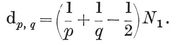
Thus the 1/N1 of 1·72 has to be replaced by d*p*, *q*/N1. (Of course the density of a convex polyhedron is 1.) We note incidentally that d*p*, *q* = d*q*, *p* : reciprocal polyhedra have the same density.
Another way of reckoning the total area of the 2N1 isosceles triangles is to observe that their angles together amount to 2d*qπ* at each vertex of {p, q}, and 2d*pπ* at the centre of each spherical {p}. Subtracting π for each triangle, we obtain the total area 2π(d*q* N0+d*p* N2−N1), whence
6·42
These two expressions for d*q*, *p*, the latter of which is a generalization of Euler’s Formula, are deducible from each other with the aid of the obvious relations
6·43
(cf. 1.71).
For the six pentagonal polyhedra 6·21, we can write N1 = 30 in 6·43 and 6·41, obtaining N2 = 60/n*p, N0 = 60/nq*, and
6·5. A digression on Riemann surfaces. The multiply-covered sphere considered above is an instance of a Riemann surface ; in fact it is a case where three or seven sheets are connected at twelve simple branch-points.
The general Riemann surface consists of an m-sheeted sphere (or m almost coincident, almost spherical surfaces) with the sheets connected at certain branch-points (or “ winding-points ”). At a branch-point of order r−1, r sheets are connected in such a way that, when we make a small circuit around the point, we pass from one sheet to another, and continue thus until all the r sheets have been taken in cyclic order. Our path is like a helix of very small pitch, save that the rth turn takes us back to the starting point. (This makes it impossible to construct an actual model without extraneous intersections of sheets.) In other words, the total angle at an ordinary point is still 2π, but the total angle at a branch-point of order r−1 is 2rπ.
The method used above, to establish 6·42, can be adapted to prove the well-known formula
6·51
for the genus of a Riemann surface.79 For this purpose, let us “ triangulate ” the Riemann surface by taking on it a sufficiently large number of points, say N0, including all the branch-points, and joining suitable pairs of them by N1 geodesic arcs so as to form N2 spherical triangles. Since the sum of all the angles of all the triangles amounts to 2π for each ordinary vertex and 2rπ for each branch-point of order r−1, the total spherical excess is
2π[N0 + Σ(r − 1)] − N2π.
Equating this to the total area 4πm, we obtain
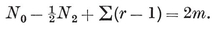
Since the faces of the map are triangles, we have 2N1 = 3N2; so

By 1·62, this is equal to 2−2p. Thus 6·51 is proved.
In particular, for any one of the Kepler-Poinsot polyhedra we have m = d*p*, *q* and Σ(r−1) = 12; so the genus is 7−d*p*, *q*. Hence (or directly from the value of N0 − N1 + N2
6·6. Isomorphism. A polyhedron may be described “abstractly ” by assigning symbols to the vertices and writing down the cycles of vertices that belong to the various faces. For instance, the cube (Fig. 3.6B) is given by the abstract description
12′34′, 2’31′4, 31′24′, 1′23′4, 23′14′, 3′12′4.
Two polyhedra that have the same abstract description (e.g. a cube and a parallelepiped) are said to be isomorphic. This means that they are topologically equivalent, or that they form the same map ; e.g., every zonohedron is isomorphic to an equilateral zonohedron (§ 2·8). Two isomorphic polyhedra evidently have the same genus, and their reciprocals are likewise isomorphic.
the dodecahedron and the great stellated dodecahedron are isomorphic. This is most easily seen by comparing the two dodecahedra of Fig. 6.6A. The first of these is repeated from Fig. 3.6E, and the second is derived by transposing any two of the symbols 1, 2, 3, 4, 5, say 4 and 5.12 34 51 23 45 in the first appears as a face of the second.
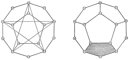
We saw, in § 3·6, that the rotation group of the dodecahedron is the alternating group on the symbols 1, 2, 3, 4, 5. (The whole group [3, 5], of order 120, is derived from this by adjoining the central inversion, which replaces each pair ij by ji.) A transposition such as (4 5) is not
consecutive sides of the faces of these polyhedra are the alternateFig. 6.2C
Table I) are derived from each other by the interchange of τπ and τ−1π.
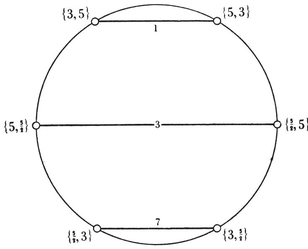
Fig. 6.6B is a scheme of the six pentagonal polyhedra, arranged round a circle. Reciprocal polyhedra are joined by horizontal lines, marked with their common density ; and isomorphic polyhedra are diametrically opposite to each other. (Cf. Fig. 14.2A.)
6·7. Are there only nine regular polyhedra?
The first and most obvious method begins with a proof that every regular polyhedron has the same vertices as a Platonic solid (and the same face-planes as a Platonic solid). For this purpose, we observe that the rotation group of {p, q} must admit an axis of n*q-fold rotation through each vertex (and an axis of np*-fold rotation through the centre of each face). But we saw in § 3·8 that the only finite rotation groups admitting more than one axis of more than 2-fold rotation are the tetrahedral, octahedral, and icosahedral groups. Thus the rotation group of {p, q} must be one of these.
Having established this lemma, we can appeal to § 6·3, where we found allbegin to construct such a polyhedron ; but it will never close up. In other words, the density is infinite, and the rotation group is not discrete.
Similar considerations enable us to assert that there are no regular star-tessellations.
This first method has involved a preliminary consideration of the Platonic solids and their rotation groups, followed by a deduction of the Kepler-Poinsot figures by faceting. It places the two sets of polyhedra in different categories. The following second method cuts across this distinction, allowing no privilege for convexity ; in fact the 9 polyhedra arise as 3+6, instead of 5+4.
If {p, q} has a finite number of edges, its Petrie polygon must have a finite number of sides ; therefore h, like p and q, must be rational. Instead of h, we use another rational number r, such that

This notation enables us to write 2·33 in the symmetrical form
6·71
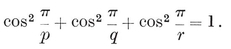
Every regular polyhedron {p, q} corresponds to a solution of this equation in rational numbers greater than 2.
There are, of course, dihedra {p, 2} (h=p) for all rational values of p; but they are not proper polyhedra, so we do not count them among the nine. There are also plane tessellations, for which r=2 and h=∞; but the present method fails to reveal those that are infinitely dense. In fact, 6·71 is a necessary but not obviously sufficient condition for {p, q} to have a finite density, and it is only by “ good fortune ” that there are no extraneous solutions with r > 2.
Gordan showed long ago80 that the only solutions of the equation
6·72

in angles commensurable with π φ1 = 2π/q, φ3 = 2π/r, we obtain, as solutions of 6·71 in rational numbers p, q, r

for which

i.e.,

In spite of its elegance, this second method suffers from two disadvantages : first, it depends on the difficult theorem that Gordan’s equation 6·72 has no further solutions ; second, it is useless for the analogous problem of regular tessellations in the plane. The following third method, like the first, is valid for plane as well as spherical tessellations.81 Moreover, it depends only on the enumeration of groups generated by reflections (§ 5·4), which is considerably easier than the more familiar enumeration of rotation groups (§ 3·8).
Consider any polyhedron {p, q}, where p and q are rational numbers greater than 2. In § 6·4 we projected its faces onto a sphere (covered d*p*, *q* times) and divided each of the spherical {p}’s into n*p* isosceles triangles. We now subdivide each isosceles triangle into two equal right-angled triangles 012, where 0 is a vertex, 1 the mid-point of a projected edge, and 2 the centre of a projected face. Clearly, the angles of such a triangle are π/q, π/2, π/p, and its sides are lines of symmetry of the spherical tessellation, as in § 4·5. The symmetry group of {p, q} is generated by reflections in these sides, and its operations transform one triangle into the whole set of 4N1 triangles, which cover the sphere d*p*, *q* times. In other words, we regard the group as operating on a Riemann surface ; if p or q is fractional, there is a branch-point of order d*p−1 or dq−1 wherever an angle π/p or π/q occurs. In this sense the triangle is a fundamental region for the group (cf. § 5·3) even when dp, q*>1. The same group, considered as operating on the single-sheeted sphere, is generated by reflections in the sides of a smaller triangle whose angles are submultiples of π, i.e., it must be one of the groups
[2, n], [3, 3], [3, 4], [3, 5],
say [m, n]. But the 4N1 small triangles (with angles π/m, π/2, π/n) cover the sphere just once, whereas the same number of large triangles (with angles π/p, π/2, π/q) cover it d*p*, *q* times. Hence each large triangle is dissected (by “ virtual mirrors ”) into exactly d*p*, *q* small triangles. (Cf. § 5·2.)
Let (x y z) denote a triangle with angles π/x, π/y, π/z. In this notation, a triangle (p 2 q) is dissected into d*p*, *q* triangles (m 2 n), so we write
(p 2 q)=d*p*, *q* (m 2 n).
The two cases
are illustrated in Fig. 6.7A
Instead of deriving the triangle (p 2 q) from a given polyhedron {p, q}, we can just as well derive the polyhedron (by Wythoff’s construction) from a suitable triangle. In the notation of § 5·7, {p, q} is

even when p or q is fractional. It remains to be seen what fractional values p and q may have.
Since repetitions of one angle of the small triangle (m 2 n) must fit into each angle of the large triangle (p 2 q), the angles π/p and π*/q* must each be a multiple of either π/m or π/n; i.e., the numerators of the rational numbers p and q must each be a divisor of either m or n. Now, if m and n are greater than 2, one of them must be 3, and the other 3 or 4 or 5. Hence, setting aside the dihedron {p, 2}, which evidently occurs for every polygon {p
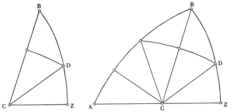
XYZ, as in Fig. 6.7B. If any set of triangles (3 2 5) form a triangle (p 2 q), where p, q are rational and greater than 2, we can take the two perpendicular sides of (p 2 q) to lie along ZX and ZY. The triangles ABZ and BCZ of Fig. 6.7A are the only possibilities. For, the three arcs AB, BC, CD, their images by reflection in YZ, ZX, XY, and the latter arcs themselves, account for all the fifteen great circles.
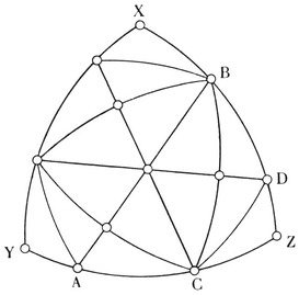
The same method can be applied to plane tessellations {p, q}, using plane triangles instead of spherical triangles. Here the group can only be [3, 6] or [4, 4] (as Δ provides no right angles, and [ ∞ ] × [ ∞ ] no acute angles), so the numerators of p and q must occur among the numbers 3, 4, 6. Thus neither p nor q can be fractional, and we see again that there are no regular star-tessellations.
We could use an analogous argument to prove that there are no regular star-honeycombs. But it is simpler to observe that, if a honeycomb {p, q, r} has cell {p, q} and vertex figure {q, r}, as in § 4·6, then the dihedral angle of the cell is 2π/r, where rTable I we see that, of the nine regular polyhedra, only the cube has such a dihedral angle. Therefore {p, q, r} can only be {4, 3, 4}.
6·8. Schwarz’s triangles. The above considerations (especially Fig. 6.7A) suggest a more general problem which was proposed and solved by Schwarz in 1873 : to find all spherical triangles which lead, by repeated reflection in their sides, to a set of congruent triangles covering the sphere a finite number of times.82 Clearly the reflections generate a group [2, n] or [3, 3] or [3, 4] or [3, 5]. Hence the sides and their transforms dissect such a triangle (p q r) into a set of congruent triangles (2 2 n) or (3 2 3) or (3 2 4) or (3 2 5). We can thus distinguish four families of “ Schwarz’s triangles ”.
Replacing each vertex in turn by its antipodes, we derive from (p q r) three colunar triangles
(p q′ r′), (p′ q r′), (p′q′ r*),*
where
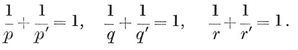
In other words, two angles are replaced by their supplements. In Table III (on page 296), colunar triangles are placed together on one line, in increasing order of size.
The largest triangles of each family, having the largest angles, are

All the others can be obtained by systematic dissection of these four in accordance with the formula
6·81
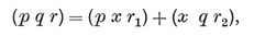

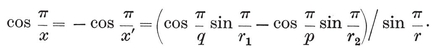
This expression for cos π/x (which is obtained by equating two expressions for cos RX in Fig. 6.8A) need never be used in practice, since the particular triangles are all visible in Fig. 4.5A on p. 66.
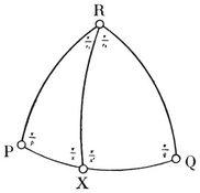
The following special cases of 6·81 will be used in § 14·8 :
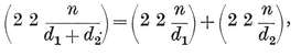
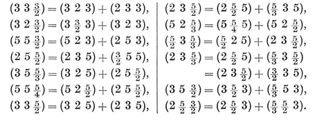
For the sake of completeness, here is another problem, analogous to Schwarz’s : to find all plane triangles which lead, by repeated reflection in their sides, to a tessellation covering the plane a finite number of times. Since any such triangle can be built up from repetitions of (3 3 3), (4 2 4), or (3 2 6), there is, besides these three, only
and this leads to a two-fold covering of the plane. (Each triangle is counted twice, with opposite orientations, and there is a simple branch-point wherever the angle 2π/3 occurs.)
6·9. Historical remarks.83 The Pythagoreans used it as a symbol of good health. 84 The systematic study of star-polygons was begun by a fourteenth-century Englishman, Bredwardin (alias l/0R)2 for a regular heptagon satisfies the equation
z3 − 7z2 + 14z − 7 = 0,
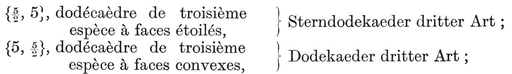
 87 Excellent photographs of them have been published by Pitsch (1, Plate I, facing p. 64) and Brückner (1, IX 1388 and XI 9). Hess and Pitsch described also their reciprocals (Brückner 1, X 28 and XI 17), whose faces are related to those of the triacontahedron in the manner of Fig. 6.9A (which is part of the drawing of the “ complete face ” in Hess 1, Fig. 3, or Bruckner 1, II 18). The rhomb 1 2 1 2 is a face of the triacontahedron itself (our Plate I, Fig. 12), 2 8 2 8 is a face of the small stellated triacontahedron (Fig. 6.4C), and 8 14 8 14 is a face of the great stellated triacontahedron. The double occurrence of the diagonals 2 2 and 8 8
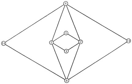
[image]
w − 2n = 2(p − 1),
[image]{.image .placeholder original-image-src=“content/images/00114” original-image-title=“” width=“0in” height=“0in”}w = Σ(r−1) and n=m.
[image]{.image .placeholder original-image-src=“content/images/00114” original-image-title=“” width=“0in” height=“0in”}p, q[image]
The third method appears to be new. Of course, the essential ideas are due to Schwarz ; but he, like Gordan, was not concerned with star-polyhedra.
Hessel (2, p. 20) observed in 1871 that the Platonic solids are not the only convex polyhedra which have equal faces and equal vertex figures. There are also the tetragonal and rhombic disphenoids : tetrahedra with isosceles or scalene faces, all alike. If we denote an isosceles triangle by {1+2} and a scalene triangle by {1+1+1}, appropriate Schläfli symbols for these disphenoids are {1+2, 1+2} and {1+1+1, 1+1+1}.
Hess (1) considered the possibility of further isohedral-isogonal polyhedra, and found, besides the Kepler-Poinsot figures, the following eight :
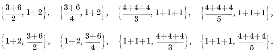
These occur in isomorphic pairs : two stellated icosahedra, two stellated triacontahedra, two faceted dodecahedra, and two faceted icosidodecahedra. The faces of the first two89 are irregular enneagrams formed by the nine points 4 and the nine points 8 in Fig. 6.2D (which is Hess’s Fig. 2 or 4). Hess remarks (p. 42) that the first has the same vertices as one of the thirteen Archimedean solids, the rhombicosidodecahedron. Of course all eight have the same symmetry group, [3, 5]. They are described in Brückner 1, pp. 207-212 ; and seven of them are shown in photographs :
IX 17,
——
XI 14,
XII 10 and 16,
XI 4 and XII 7,
XII 11 and 17,
XII 8 and 20,
XII 12 and 21.
In a later work Brückner went further and found many other such polyhedra. These, however, could be excluded by making some quite natural restrictions ; e.g., in one case (Brückner 2, p. 161) the face is a hexagram two of whose vertices coincide !
[]
¶ CHAPTER VII
ORDINARY POLYTOPES IN HIGHER SPACE
POLYTOPE is the general term of the sequence
point, segment, polygon, polyhedron, . . . .
[image]{.image .placeholder original-image-src=“content/images/00114” original-image-title=“” width=“0in” height=“0in”}α3, β3, γ3, and δ3 for the tetrahedron, octahedron, cube, and “ squared paper ” tessellation, and define the general αn, βn, γn, δn[image]{.image .placeholder original-image-src=“content/images/00114” original-image-title=“” width=“0in” height=“0in”}not[image]{.image .placeholder original-image-src=“content/images/00114” original-image-title=“” width=“0in” height=“0in”}n-dimensional Schläfli symbol, which enables us to read off many properties of a regular polytope at a glance ; e.g., the elements of {p, q, r, … }, besides vertices and edges, are plane faces {p}, solid faces {p, q}, and so on. (The number of digits p, q, r[image]{.image .placeholder original-image-src=“content/images/00114” original-image-title=“” width=“0in” height=“0in”}p, q, r,[image]{.image .placeholder original-image-src=“content/images/00114” original-image-title=“” width=“0in” height=“0in”}n[image]{.image .placeholder original-image-src=“content/images/00114” original-image-title=“” width=“0in” height=“0in”}p, q, r, … , and see why {p, q, r, …} reciprocates into {. . . , r, q, p[image]
[image]{.image .placeholder original-image-src=“content/images/00114” original-image-title=“” width=“0in” height=“0in”} There are three ways of approaching the Euclidean geometry of four or more dimensions : the axiomatic, the algebraic (or analytical), and the intuitive. The first two have been admirably expounded by Sommerville and Neville, and we shall presuppose some familiarity with such treatises.90 Concerning the third, Poincaré wrote,
Un homme qui y consacrerait son existence arriverait peut-être à se peindre la quatrième dimension.
Only one or two people have ever attained the ability to visualize hyper-solids as simply and naturally as we ordinary mortals visualize solids ; but a certain facility in that direction may be acquired by contemplating the analogy between one and two dimensions, then two and three, and so (by a kind of extrapolation) three and four. This intuitive approach91 is very fruitful in suggesting what results should be expected. However, there is some danger of our being led astray unless we check our results with the aid of one of the other two procedures.
For instance, seeing that the circumference of a circle is 2πr, while the surface of a sphere is 4πr2, we might be tempted to expect the hyper-surface of a hyper-sphere to be 6πr3 or 8πr3. It is unlikely that the use of analogy, unaided by computation, would ever lead us to the correct expression, 2π2r3.
Many advocates of the intuitive method fall into a far more insidious error. They assume that, because the fourth dimension is perpendicular to every direction known through our senses, there must be something mystical about it.92 Unless we accept Houdini’s exploits at their face value, there is no evidence that a fourth dimension of space exists in any physical or metaphysical sense. We merely choose to enlarge the scope of Euclidean geometry by denying one of the usual axioms (“ Two planes which have one common point have another ”), and we establish the consistency of the resulting abstract system by means of the analytical model wherein a point is represented by an ordered set of four (or more) real numbers : Cartesian coordinates.
Little, if anything, is gained by representing the fourth Euclidean dimension as time. In fact, this idea, so attractively developed by H. G. Wells in The Time Machine, has led such authors as J. W. Dunne (An Experiment with Time) into a serious misconception of the theory of Relativity. Minkowski’s geometry of space-time is not Euclidean, and consequently has no connection with the present investigation.
After these words of warning, we proceed to describe some of the simplest polytopes, following the intuitive approach so far as is safe, and utilizing coordinates whenever they help to clarify the subject.
[image]{.image .placeholder original-image-src=“content/images/00114” original-image-title=“” width=“0in” height=“0in”}. In space of no dimensions the only figure is a point, II0. In space of one dimension we can have any number of points ; two points bound a line-segment, Π1, which is the one-dimensional analogue of the polygon Π23011 to a third point (outside its line) we construct a triangle,2. By joining the triangle to a fourth point (outside its plane) we construct a tetrahedron,3. By joining the tetrahedron to a fifth point (outside its 3-space !) we construct a pentatope,4. (See Fig. 7.2A.) The general case is now evident : any n+1 points which do not lie in an (n−1)-space are the vertices of an *n-*dimensional simplex, whose elements are simplexes formed by subsets of the n n+1 cells : in a single formula,
[image]
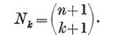
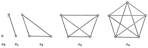
FIG. 7.2A: Simplexes
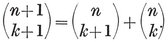 k-dimensional elements belong to the base, while others are pyramids erected on (k−1)-dimensional elements of the base.
A line-segment is enclosed by two points, a triangle by three lines, a tetrahedron by four planes, and so on. Thus the general simplex may alternatively be defined as a finite region of n-space enclosed by n+1 hyperplanes or (n−1)-spaces.
 regular simplex, which we shall denote by α*n*. Thus
α0 = Π0, α1 = Π1, α2 = {3}, α3 = {3, 3}.
Fig. 7.2A shows a sort of perspective view of these simplexes. The equilateral triangle α2 has been deliberately foreshortened to emphasize its occurrence as a face of α3.
One of the fundamental properties of n-dimensional space is the possibility of drawing n mutually perpendicular lines through any point O; n points equidistant from O along these lines are evidently the vertices of a simplex αn−1. Producing the lines beyond O, we obtain a Cartesian frame or cross. Points equidistant from O in both directions are the 2n vertices of another important figure, the cross polytope βn, whose cells consist of 2*n* αn−1’s. Thus
β1 = Π1, β2 = {4}, β3 = {3, 4}.
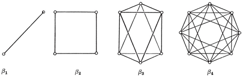
FIG. 7.2B: Cross polytopes
The octahedron β3 is an ordinary dipyramid based on β2 ; similarly β4 is a four-dimensional dipyramid based on β3 (with its two apices in opposite directions along the fourth dimension). The β3 of Fig. 7.2B is not an orthogonal projection of the octahedron but an oblique (parallel) projection, to emphasize its occurrence as base of the dipyramid β4.
Since βn is a dipyramid based on βn−1, all its elements are either elements of β*n*−1 or pyramids based on such elements. Thus all are simplexes, and the number of α*k’s in βn* is
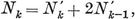
k’s in βn−1 (which vanishes when k=n−1). Also N0=2n. It is now easily proved by induction that
[image]
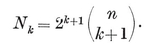
n into n−1.) Thus β4 has 8 vertices, 24 edges, 32 plane faces, and 16 cells.
The derivation of α*n*−1 and βn from a cross shows that the permutations of
[image]
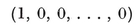
are coordinates for the vertices of an α*n*−1 of edge √2, lying in the hyperplane Σ*x* = 1, and that the permutations of
[image]
are coordinates for the vertices of a β*n* of edge √2.
011 is translated (not along its own line) from an initial to a final position, it traces out a parallelogram. Similarly a parallelogram traces out a parallelepiped. The n-dimensional generalization is known as a parallelotope. It has 2*n* vertices. The remaining elements are k-dimensional parallelotopes. Their number, Nk93 Since
we easily prove by induction that
[image]
Thus the four-dimensional parallelotope (the γ4 of Fig. 7.2C) has 16 vertices, 32 edges, 24 faces, and 8 cells. (It is instructive to look for the eight parallelepipeds in the figure, and to observe how each parallelogram belongs to two of them.)
The n translations used in constructing the parallelotope define n vectors, represented by the n edges that meet at one vertex. In other words, all the vertices are derived from a certain one of them by applying all possible sums of these n vectors, without repetition. Similarly, by applying all possible sums of all integral multiples of the n vectors, we obtain the points of an n-dimensional lattice, which are the vertices of a special n-dimensional honeycomb whose cells are equal parallelotopes.
If the n vectors are mutually perpendicular (as of course they can be, in n dimensions), the parallelotope is an orthotope, the generalization of the rectangle and the “ box ”. If the n perpendicular vectors all have the same magnitude, the orthotope is a hyper-cube or measure polytope, γ*n, and the corresponding lattice determines the cubic honeycomb, δn+1, of which the three-dimensional case (δ4[image]{.image .placeholder original-image-src=“content/images/00114” original-image-title=“” width=“0in” height=“0in”}*n*+1 rather than δn*, because of the resemblance between n-dimensional honeycombs and (n+1)-dimensional polytopes (e.g., between plane tessellations and polyhedra) ; in fact, we regard honeycombs as “ degenerate ” polytopes. Thus
[image]

[image]
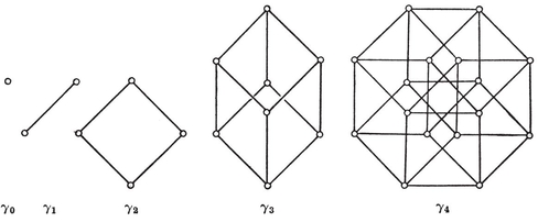
FIG. 7.2C: Measure polytopes
The name “ measure polytope ” is suggested by the use of the hyper-cube of edge 1 as the unit of content (e.g., the square as the unit of area, and the cube as the unit of volume). The usual processes of the integral calculus extend in a natural manner ; e.g., the content of an n-dimensional pyramid is one nth of the product of base-content and altitude.
We have constructed the *n-*dimensional orthotope by translating the (n−1) -dimensional orthotope along a segment in a perpendicular direction. Clearly, the same process may be applied to any (n−*n*−1*n*−111*n*−1 (including the interior). Accordingly, we call the generalized prism the rectangular product*n*−11, and use the symbol
*n*−11.
More generally,94jk, in completely orthogonal spaces, determine a (j + kjkkj). In particular, the product of a p-gon and a q-gon is a four-dimensional figure whose cells consist of q p-gonal prisms and p q-gonal prisms. An intuitive idea of this may be acquired as follows.
Let q solid p-gonal prisms be piled up, base to base, so as to form a column. In ordinary space the base of the lowest prism and the top of the highest are far apart. But in four-dimensional space, where rotation takes place about a plane (instead of about a point or a line, as in two or three dimensions), we can bring these two p-gons into contact by bending the column about the planes of the intermediate bases. The column is thus converted into a ring, whose surface consists of pq rectangles. Another such ring can be made from p q-gonal prisms. If the lengths of the edges are properly chosen (e.g., if they are all equal), the two rings can be interlocked in such a way that the two sets of pq rectangles (or squares) are brought into coincidence. There are then no external faces, and we have constructed the rectangular product of two polygons. In particular, the rectangular product of two rectangles is the four-dimensional orthotope, and the rectangular product of two equal squares is the hyper-cube :
γ2 × γ2 = γ4.
More generally,
γ*j* × γ*k* = γ*j*+*k*.
k is itself a rectangular product of two figures, then Π*j* × Π*k* is a rectangular product of three figures, which may be taken in any order; for this kind of “multiplication” is associative as well as commutative. Similarly we may define the rectangular product of any number of figures. In particular, the rectangular product of n segments is an n-dimensional orthotope, and that of n equal segments is the n-dimensional measure polytope :
γ1n = γ*n*.
More generally,
γ*j* × γ*k* × . . . = γj+*k*+ . . . .
[image]{.image .placeholder original-image-src=“content/images/00114” original-image-title=“” width=“0in” height=“0in”}. The word sphere (rather than “ hypersphere ”) is generally used for the locus of a point at constant distance r from a fixed point; thus a one-dimensional sphere is a point-pair, and a two-dimensional sphere is a circle. (Topologists, being more concerned with the dimension-number of the locus itself than with that of the underlying space, prefer to call the point-pair a 0-sphere, the circle a 1-sphere, and so on.) Let Sn denote the (n−1)-dimensional content or “surface” of an n-dimensional sphere of unit radius ; e.g., S1 = 2, S*2* = 2π. Then the “surface” of a sphere of radius r is, of course, Snrn-1, and the n-dimensional content or “volume” of a sphere of radius R is
[image]
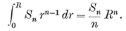
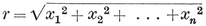 n-dimensional space, we may take the element of content to be either dx1 dx2 . . . dxn or Sn rn−1 dr. An expression for Sn (as a function of n
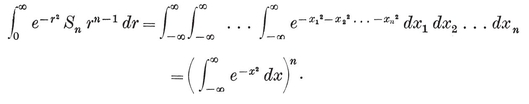
But the integrals involved are gamma functions : in fact,
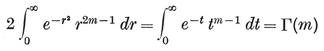
and
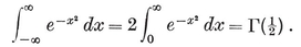
Hence
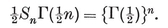
Since S2=2π, the case when n
7.32
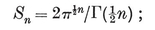
e.g., S4=2π2. Since Γ(m+1)=mΓ(m), it follows from 7·31 that the n-dimensional content (for radius R) is
7·33
The particular values of Sn are very easily computed with the aid of the recurrence formula
Sn+2 = 2πS*n*/n,
which states that the (n+1)-dimensional content of the (n+2)-dimensional unit sphere is 2π times the n-dimensional content of the n-dimensional unit sphere ; e.g., S2/2=π S4=2π2
With respect to the sphere x12 + . . . + xn2 = r2, any point (y1, . . . , yn) (other than the centre, which is the origin) has a polar hyperplane y1x1 + . . . + ynxn = r2, which is a tangent hyperplane if the point (pole) lies on the sphere. If j points determine a (j−1)-space, their j polar hyperplanes intersect in a polar (n−j)-space. It is easily seen (as in two or three dimensions) that the relation between two such polar spaces is symmetric.
On comparing 7·22 with 7·25, we find that the value of Nn−*j* for yn is the same as the value of Nj−1 for βn βn and yn are reciprocal polytopes : the vertices of either are the poles of the bounding hyperplanes of the other, with respect to a concentric sphere ; consequently the (j*j*−1’s of the one, being determined by sets of j vertices, correspond to the (n−j*n*−*j*’s of the other, which are determined by sets of j intersecting hyperplanes. In fact, the sphere x12+ . . . + xn2 = 1 reciprocates the 2n vertices 7·24 of βn into the 2n hyperplanes
x1 = ± 1, . . . , xn = ± 1,
which bound the yn (of edge 2) whose 2*n* vertices are
7·34
Similarly, an is self-reciprocal (or, rather, reciprocates into another an), in agreement with the fact that Nn−*j*=Nj−1. (See 7·21.)
7·4. Polytopes and honeycombs. After the introductory account of special cases in § 7·2, we are now ready for the formal definition of a polytope. For simplicity, we assume convexity until we come to Chapter XIV. (A region is said to be convex if it contains the whole of the segment joining every pair of its points.) Accordingly, we define a polytope as a finite convex region of n-dimensional space enclosed by a finite number of hyperplanes. If the space is Euclidean (as we shall suppose until § 7·9), the finiteness of the region implies the inequality
Nn*−1**>*n
for the number of bounding hyperplanes.
n is the set of all points whose Cartesian coordinates satisfy Nn−1 linear inequalities
bk1 x1 + bk2 x2 + . . . + bkn xn ≤ bk0 (k = 1, 2, . . ., Nn−1);
which are consistent but not redundant, and provide the range for a finite integral
(the content of the polytope). The part of the polytope that lies in one of the hyperplanes is called a cell. Since one of the inequalities is here replaced by an equation, each cell is an (n*n*−1*n*−1*n*−2’s, and so on ; we thus obtain a descending sequence of elements*n*−1*n*−2, . . .,10*n*−2*n*−1’s.
43210. It differs from a three-dimensional honeycomb (§ 4·6) in having a finite number of elements.
An n*n*+1n’s fitting together to fill nnn.
*n*−*j**j*−1’s, as in § 7·3. Whenever the given polytope has a special interior point which can be called its centre, we naturally choose this same centre for the reciprocating sphere. We can then speak of the reciprocal polytope, as its shape is definite (though of course its size changes with the radius of reciprocation). In particular, if there is a sphere which touches all the cells, then the points of contact (which are the “ centres ” of the cells) are the vertices of the reciprocal polytope. By analogy, if the cells of a honeycomb have centres, we define the reciprocal honeycomb as having those centres for its vertices. For instance, the δn+1 whose vertices have n even coordinates (in every possible arrangement) is reciprocal to the δn+1 whose vertices have n odd coordinates.
It is natural to regard an n-dimensional polytope as having one n-dimensional element, namely itself; so we write
Nn = 1.
Reciprocation converts this into the less obvious convention95
N−1 = 1.
Both formulae are in agreement with 7·21; but 7·22 holds only for k<n, and 7·25 only for k≥0. We observe incidentally that, with these reservations, Nk for αn is the coefficient of Xk+1 in (1+X)*n*+1, Nk for βn is the coefficient of Xk+1 in (1+2X)n, and Nk for yn is the coefficient of Xk in (2+X)n. Hence 96
7·41
in the three respective cases. We shall make use of these expressions in § 9·1.
7·5. Regularity. If the mid-points of all the edges that emanate from a given vertex O*n* lie in one hyperplane (e.g., if there are only n such edges, or if all the vertices lie on a sphere and all the edges are equal), then these mid-points are the vertices of an (n−1)-dimensional polytope called the vertex figuren. at O. Its cells evidently are the vertex figures (at O*n* which surround O. (Cf. §§ 2·1, 4·6.)
n (n>2) is said to be regular if its cells are regular and there is a regular vertex figure at every vertex. By a natural extension of the argument used in § 2·1, the cells are all equal, and the vertex figures are all equal. (The equality of vertex figures is actually easier to establish in four dimensions than in three !) For instance, the polytopes
αn, βn, yn
are regular, with cells αn−1, αn−1, yn−1, and vertex figures αn−1, βn−1, αn—1.
There are, of course, several other possible definitions for a regular polytope. The one chosen has the advantage of simplicity. (We do not need to assume equality of cells, or of vertex figures.) But admittedly it has the disadvantage of applying only in more than two dimensions : a0, a1, and {p} have to be declared regular by a special edict.
The same definition of regularity can be used for a honeycomb, though it is simpler to say (as in § 4·6) that a honeycomb is regular if its cells are regular and equal. For instance, δn+1 is regular, with cells yn and vertex figures βn.
4 whose cells are {p, q} must have vertex figures {q, r}. (Here r is simply the number of cells that surround an edge.) Accordingly, we write
4 = {p, q, r};
e.g.,
α4 = {3, 3, 3}, β4 = {3, 3, 4}, y4 =
5 whose cells are {p, q, r} must have vertex figures {q, r, s}, and we write
5 = {p, q, r, s}.
The same kind of symbol will describe a four-dimensional honeycomb. Finally, the general regular polytope or honeycomb {p, q, . . . , v, w} has cells {p, q, . . . , v} and vertex figures {q, … , v, w}. (Of course, both {p, q, … , v} and {q, … , v, w} must be polytopes, even if {p, q, . . . , v, w} itself is a honeycomb.) In particular, for any n> 1,
Carrying this notation back to one dimension, we write
a1 = { }.
The only “ misfit ” is δ2 = { ∞ }.
7·6. The symmetry group of the general regular polytope. If we are given the position in space of one cell and one vertex figure, we can build up the whole polytope, cell by cell, in a perfectly definite manner. The various cells are not merely equal but equivalent, i.e., there is a symmetry group which is transitive on the cells, and likewise transitive on the vertices. In particular, the symmetry group of the regular simplex an is the symmetric group of degree n+1, viz., the group of all permutations of the n+1 vertices (or of the n+1 cells).
Since Theorem 3·41 is valid in any number of dimensions, it follows that every regular polytope has a centre O*n, around which we can draw a sphere of radius jR through the centres of all the Πj*’s, for each value of j from 0 to n−1. The first and last of these concentric spheres are, of course, the circum-sphere and the in-sphere.
We proceed to describe the “simplicial subdivision ” of a regular polytope, beginning with the one-dimensional case. The segment Π1 is divided into two equal parts by its centre O1. The polygon Π2={p} is divided by its lines of symmetry into 2p right-angled triangles, which join the centre O2 to the simplicially subdivided sides. The polyhedron Π3={p, q} is divided by its planes of symmetry into g quadrirectangular tetrahedra (see 5·43), which join the centre O3 to the simplicially subdivided faces. Analogously, the general regular polytope Π*n* is divided into a number of congruent simplexes (of a special kind) which join the centre O*n* to the simplicially subdivided cells. A typical simplex is O0 O1 … O*n, where Oj* is the centre of a cell of the Π*j*+1 whose centre is O*j*+1 (j=0, 1, … , n−1). In other words, O*n*−1 is the centre of a cell of Π*n*, O*n*−2 is the centre of a cell of that cell, … , O1 is the mid-point of an edge, and O0 is one end of that edge. The edge { } is thus divided into N10=2 segments, the plane face {p} into N21 N10 triangles, the solid face {p, q} into N32 N21 N10 tetrahedra, … , and the whole polytope {p, q, … , v, w} into
gp, q, . . . , v, w = Nn−1 Nn−1, n−2 . . . N21 N10
simplexes. (The “ configurational numbers ” Njk or Nj,k were defined in § 1·8. An element Π*j* belongs to Njk Π*k’s for each k>j, and contains Njk Πk*’s for each k<j.)
This number gp, *q*, …, *v*, *w* is an important property of the polytope {p, q, . . . , v, w}. In fact, it is the order of the symmetry group [p, q, . . . , v, w]. We prove this by induction, beginning with the obvious fact that the symmetry group of the one-dimensional polytope { } has order N0=2. We assume the corresponding result in n−1 dimensions, so that the symmetry group of a cell {p, q, … , v} has order
7·61
In the symmetry group of the whole polytope, this occurs as a subgroup of index Nn−1, viz., the subgroup leaving O*n*−1 invariant. (The Nn−1 cosets correspond to the Nn−1 cells.) Hence gp, q, . . . , v, w is the order of the whole group.
An alternative expression for this number is obtained from the subgroup of index N0 which leaves a vertex O0 invariant. This, being the symmetry group of the vertex figure {q, … , v, w}, has order
7·62
By repeated application of this equation, we find
gp, q, …, v, w = N0 N01 N12 … Nn−2, n−1.
(Of course Nn−2, *n*−1 = 2.)
Just as the vertex figure {q, r, … , w} indicates the way a vertex is surrounded, so the “ second vertex figure ” {r, … , w} (which is the vertex figure of the vertex figure) indicates the way an edge is surrounded. Thus the subgroup of [p, q, r, … , w] that leaves an edge absolutely invariant is [r, … , w], of order gr, . . . , *w*. But there is also a subgroup of order 2 that interchanges the ends of the edge (viz., a subgroup isomorphic with the symmetry group of the edge itself). The complete subgroup leaving O1 invariant is the direct product of these two. Hence
2gr, . . . , w = gp, q, r, . . . , w*/N1.*
The general situation is now clear : the number of elements {p, … , r} in the regular polytope {p, … , r, s, t, u, … , w} is
7·63
For, the subgroup leaving such an element invariant as a whole is the direct product
[p, . . . , r] × [u, . . . , w],
where the first factor is isomorphic with the symmetry group of that element, while the second leaves the element absolutely invariant. In the case of an, the g’s are factorials, and we have
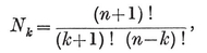
in agreement with 7·21.
When n=2, 3, and 4, we have, respectively,
N1 = N0 = gp/2*,* where gp = 2p,
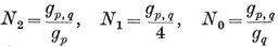
, where
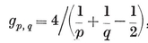
, and
7·64
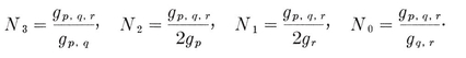
But there is no simple expression for gp, q, r as a function of p, q, r.
The three-dimensional case may be written
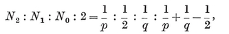
in agreement with Euler’s Formula N2 + N0 − N1 = 2. Applying
to the cell and vertex figure of the four-dimensional polytope {p, q, r}, we obtain
Since N13=r=N12 and N21=p=N20, we can use 1·81 to show that
N3 N31 = N1 r = N2 p = N0 N02,
whence97
7·65
in agreement with 7·64. It follows that
N3 + N1 = N2 + N0;
but this relation, unlike 1·61, is homogeneous, and so does not provide an expression for gp, q, r.
In fact, the most practical way to determine N0 or N3 (and thence gp, q, r) is by actually counting the vertices or cells of each four-dimensional polytope. This is not too laborious, provided we count them in reasonably large batches, as in Chapter VIII. On the other hand, it seems more mathematically satisfying to compute than to count, so we shall give a general formula in § 12·8.
The symmetry groups of the regular simplex and cross polytope may be considered separately, as follows. Since the symmetry group of an or {3*n*−1} is the symmetric group of degree n+1, we have
7·66
Since βn or {3*n−*2, 4} has 2*n* cells an−1, 7·61 shows that
7·67
In fact, the symmetry group of βn (or of γn) is just the symmetry group of the frame of orthogonal Cartesian axes, and so consists of the 2*n* possible changes of sign of the n coordinates, combined with the n ! permutations of the axes.
7·7. Schläfli’s criterion. The angles
φ = O0 O*n* O1, χ = O0 O*n* O*n*−1, ψ = O*n*−2 O*n* O*n*−1
are the natural generalization for the angles φ, χ, ψ defined in § 2·4. We still have
7·71
2φ is the angle subtended at the centre by an edge (of length 2l), χ is the angle subtended by the circum-radius of a cell, and π−2ψ is the dihedral angle (between the hyperplanes containing two adjacent cells).
We proceed to find a general formula for the property φ of {p, q, … , v, w}, and a necessary condition for the existence of such a polytope.
Letting 0R′, l′, φ′ denote the values of 0R, l, φ for the vertex figure {q, … , v, w}, we have
0R′ sin φ′ = l′ = l cos π/p
and, from Fig. 2.4B (with O*n* instead of O3), 0R′=l cos φ. Hence
7·72
i.e.,
If φ″ refers to the “ second vertex figure,” and φ(*k*) to the “ kth vertex figure,” we have similarly98
But φ(*n*−2) = π/w. Hence
7·73
where the Δ-function is determined by the recurrence formula
7·74
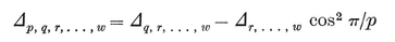
with the initial cases
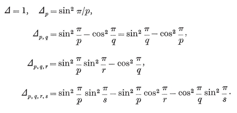
It is easily proved by induction that
7·75
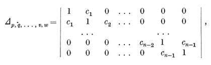
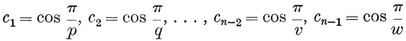
Δw, v, . . ., q, p = Δp, q, . . . , v, w.
Another explicit formula is
7·76

where
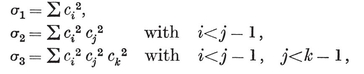
and so on. (We shall have occasion to generalize both the determinant and the series, in § 12·3.) In particular,99
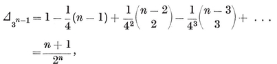
whence, by 7·74,
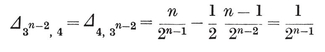
and
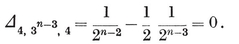
By repeated application of 7·73, we have
sin2 φ sin2 φ′ … sin2 φ(*n−*2) = Δp, q, . . ., *v*, *w*.
Hence
7·77
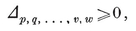
with the strict inequality for a finite polytope, and the equality for a honeycomb (where 0R = ∞ and φ=0). This is “Schläfli’s criterion ” for the existence of a regular figure corresponding to a given symbol {p, q, . . . , v, w}.
When n=3, we have Δp, q ≥ 0, which is equivalent to

This inequality, multiplied through by π, simply states that the triangle P0 P1 P2 of 2·52 has the proper angle-sum to be spherical or Euclidean.
When n=4, we have Δp, q, r ≥ 0, or
7·78
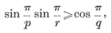
which states that 2π/r is greater than or equal to the dihedral angle π−2ψ of {p, q}. (See 2·44.) In other words, it states the possibility of fitting r {p, q}’s round a common edge.100
When n=5, we have Δ*p, q, r, s* ≥ 0, or
7·79
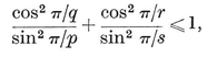
which states that the values of ψ for {p, q} and {s, r} are together greater than or equal to π/2. (A geometrical reason for this will be seen later.)
7·8. The enumeration of possible regular figures. When n=4, we have a Schläfli symbol {p, q, r}, where both {p, q} and {q, r} must occur among the Platonic solids
{3, 3}, {3, 4}, {4, 3}, {3, 5}, {5, 3}.
The criterion 7·78 admits the six polytopes
7.81

and the one honeycomb {4, 3, 4}, but rules out
7·82

Then the criterion 7·79 admits the three polytopes
7·83

and the three honeycombs
7·84
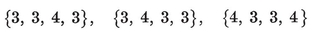
(of which the last is δ5), but rules out
7·85

Since the only regular polytopes in five dimensions are α5, β5, γ5, it follows by induction that in more than five dimensions the only regular polytopes are αn, βn, γn, and the only regular honeycomb is δ*n*+1.
Since 7·77 is merely a necessary condition, it remains to be proved that the four-dimensional polytopes {3, 4, 3}, {3, 3, 5}, {5, 3, 3} and honeycombs {3, 3, 4, 3}, {3, 4, 3, 3} actually exist. This is usually done by building up the polytopes, cell by cell, an exceedingly laborious process in the case of {3, 3,. 5} or {5, 3, 3}.101
Two superior methods of construction will be described : one in §§ 8·2-8·5, and the other in § 11·7.
7·9. The characteristic simplex. What kind of figure is the simplex O0 O1 . . . O*n* of § 7·6 ? We defined O*j* as the centre of a cell Π*j* of the Π*j*+1 whose centre is O*j*+1. Hence O*j*+1 O*j* is perpendicular to the j-space of the Π*j*, and all the lines
O*n* O*n*−1, O*n*−1 O*n*−2, . . . , O2 O1, O1 O0
are mutually perpendicular. In fact, each triangle O*i* O*j* O*k* (i<j<k) is right-angled at O*j. Thus the j-space O0 O1 . . . Oj* is completely orthogonal to the (n−j)-space O*j* O*j*+1 … O*n. It follows that the hyperplanes O0 . . . O*k−*1 O*k*+1 . . . On* and O0 . . . O*i−*1 O*i*+1 . . . O*n, which contain these respective subspaces, are perpendicular (provided i<j<k). In other words, the dihedral angle opposite to the edge Oi* O*k* is a right angle whenever i<k−1. Such a simplex is called an orthoscheme ; e.g., O0 O1 O2 O3 is a quadrirectangular tetrahedron.
The lines O*n* O*j* (j=0, 1, . . . , n−1 which are “radii” of Π*n, meet the unit sphere round On* in points P*j* which form a spherical simplex102 P0 P1 . . . P*n*−1. (See 2·52 for the case when n=3.) Such simplexes cover the sphere, and there is one for each operation of the symmetry group [p, q, . . . , v, w]. Thus the characteristic simplex P0 P1 . . . P*n*−1 is a fundamental region for the group. The reciprocal polytope naturally has the same symmetry group ; it also has the same characteristic simplex, with the P’s named in the reverse order.
The dihedral angle of O0 O1 . . . O*n* opposite to the edge O*i* O*k* (i<k<n) is the same as the dihedral angle of P0 P1 . . . P*n−*1 opposite to P*i* P*k. Hence (or by a direct argument similar to that used for O1 O1 . . . On* above) the characteristic simplex is a spherical orthoscheme. We shall soon find that its acute dihedral angles, opposite to the edges
P0 P1, P1 P2, . . . , P*n*−2 P*n−*1,
are
π/p, π/q, . . . , π/w.
For this purpose it is desirable to project the polytope radially onto a concentric sphere, so as to obtain a partition of the sphere into Nn−1 spherical polytopes, which we regard as the cells of a spherical honeycomb. The spherical honeycomb shares all the numerical properties of the polytope, and also, when properly interpreted, its angular properties. Pairs of adjacent vertices are joined, not by Euclidean straight segments, but by arcs of great circles (which are the straight lines of “ spherical space ”). These “edges” are of length 2P0 P1 = 2φ. The cells are (n−1)-dimensional spherical polytopes of circum-radius P0 P*n*−1=χ and in-radius P*n*−2 P*n*−1=ψ.
We allow the Schläfli symbol {p, … , v} to have three different meanings : a Euclidean polytope, a spherical polytope, and a spherical honeycomb. This need not cause any confusion, so long as the situation is frankly recognized. The differences are clearly seen in the concept of dihedral angle. The dihedral angle of a spherical polytope is greater than that of the corresponding Euclidean polytope, but a spherical honeycomb has no such thing (save in a limiting sense, where we might call it π). An infinitesimal spherical polytope is Euclidean ; and as the circum-radius of a spherical polytope increases from 0 to π/2, the dihedral angle increases from its Euclidean value to π, the final product being a spherical honeycomb.
For instance, {4, 3}, qua Euclidean polytope, is an ordinary cube (of dihedral angle π/2), which may be a cell of the Euclidean honeycomb {4, 3, 4}. Qua spherical polytope (on a sphere in four dimensions) its faces are spherical quadrangles, and its dihedral angle may take any value between π/2 and π ; in particular, when the dihedral angle is 2π/3, the spherical hexahedron is of the right size to be a cell of the spherical honeycomb {4, 3, 3}. Finally, qua spherical honeycomb it covers a sphere in ordinary space, and its faces are spherical quadrangles of angle 2π/3.
The arrangement of characteristic simplexes covering the sphere can be obtained directly as a simplicial subdivision of the spherical honeycomb. In fact, P*n*−1 is the centre of a cell, P*n*−2 is the centre of a cell of that cell, and so on. From the corner P*n*−1 of the characteristic simplex P0 P1 . . . P*n*−1 of {p, q, . . . , v, w}, a small sphere with centre P*n*−1 P*n*−1 P*i) which is similar to the characteristic simplex of the cell {p, q, … , v}. Again, from the corner P0 a small sphere with centre P0
 P0 P*i*+1) similar to the characteristic simplex of the vertex figure {q, … , v, w}.*
The characteristic simplex of {p} is an arc P0 P1 of length
φ*p* = χ*p* = ψp = π/p.
That of {p, q} is a spherical triangle P0 P1 P2, with angles π/q, π/2, π/p at the respective vertices, and sides
P0 P1 = φ*p, q, P0 P2 = χp, q, P1 P2 = ψp, q*,
whose trigonometrical functions can be read off from Fig. 2.4A.
The characteristic simplex of {p, q, r} is a quadrirectangular spherical tetrahedron P0 P1 P2 P3 (cut out from a sphere in four dimensions by four hyperplanes through the centre O4), whose solid angles at the vertices P3 0and P0 correspond to the characteristic triangles of {p, q} and {q, r}. (See Fig. 7.9A.) Thus the dihedral angles at the edges P2 P3, P0 P3, P0 P1 are
πlp, πlq, π*/*r,
while the remaining three are right angles.103 Also the face-angles at the vertices P3, P0 are
∠P0 P3 P1 = **φp,q′
**∠P1 P0 P2 = φq,r′
∠P0 P3 P2 = χp,q′
∠P1 P0 P3=χq,r′
∠P1 P3 P2 = ψp,q′
∠P2 P0 P3 = ψq,r′
and the remaining acute angles, being equal to dihedral angles, are
∠P0 P2 P1= π/p, ∠P2 P1 P3 = πlr .
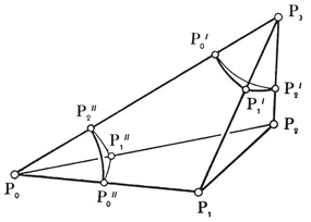
Hence, from the right-angled spherical triangles P0 P1 P2, P0 P1 P3, P1 P2 P3,
[image]
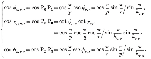
We have seen that the characteristic simplex of {p, q, . . . v, w}, being a spherical orthoscheme, has dihedral angles π/2 opposite to all its edges except
P0 P1,P1 P2,…, P*n–*2 P*n–*1.
We are now ready to prove that the remaining dihedral angles are
π/p, π/q, …, π/w.
This statement has already been verified in 2, 3, and 4 dimensions ; so let us assume it for *n—*1 dimensions and use induction.
π/p, π/q, . . . , π/v
 ;
;
π/q, π/r, . . . , π/w
 P0 P1. . . Pn−1** opposite to Pi** Pj** (i<j<n−1
 0 P1. . .P*n*−1 opposite to P*i*+1P*J*+1
 P0 P1. . . P*n−**1*** has the dihedral angles π/p, π/q, . . . , π/v, π/w, as required.
Since the reciprocal honeycomb has the same P’s in the reverse order, it follows that
The reciprocal of {p, q, … , v, w} is {w, v, … , q, p}.
Most of the above theory applies to Euclidean honeycombs just as well as to spherical honeycombs. The characteristic simplex P0 P1. . .Pn−1** (or O0 O1. . . On−1**) is then a Euclidean orthoscheme, the fundamental region for the infinite symmetry group.
[image]
[image]
Since ψ*p*,*q* = ∠ P1 P3 P2 and π/r = ∠P3 P1 P2, this simply means that the angle-sum of the right-angled triangle P1 P2 P3 is greater than or equal to π. Exactly the same interpretation can be given to the inequality
[image]
which comes from 7.79. For, in the orthoscheme P0 P1 P2 P3 P4 ∠P3 P1 P2=ψ[image]
The angles φ and φ are reciprocal properties, in the sense that
φw, . . . p = ψp, . . . ,w.
[image]
[image]
This provides an expression for the dihedral angle π—2ψ of the Euclidean polytope {p, q, … , v, w}. We might expect to find a new criterion by remarking that a known polytope {p, q, . . . , v} can serve as the cell of a possible polytope or (Euclidean) honeycomb {p, q, . . . , v, w} provided w repetitions of its dihedral angle can be fitted into a total angle of 2π, i.e., provided


[image]{.image .placeholder original-image-src=“content/images/00114” original-image-title=“” width=“0in” height=“0in”} Practically all the ideas in this chapter (with the exception of Schoute’s generalized prism or rectangular product, described on page 124) are due to Schläfli, who discovered them before 1853—a time when Cayley, Grassmann, and Möbius were the only other people who had ever conceived the possibility of geometry in more than three dimensions.104
Observing that gp, . . . , w is equal to the number of repetitions of the spherical orthoscheme P0 P1 . . . P*n*−1 that will suffice to cover the whole sphere, Schläfli investigated the content of such a simplex as a function of its dihedral angles. He showed how this function can be defined by a differential equation, and obtained many elegant theorems concerning it. In the four-dimensional case (where the differential equation was rediscovered fifty years later by Richmond), he denoted the volume of the quadrirectangular tetrahedron P0 P1 P2 P3 by
It seems105 that the simplest explicit formula for this “ Schälfli function ” is
where
[image]{.image .placeholder original-image-src=“content/images/00114” original-image-title=“” width=“0in” height=“0in”}gp,q,r (although this will not throw any further light on the volume of a spherical tetrahedron).
Ludwig Schläfli was born in Grasswyl, Switzerland, in 1814. In his youth he studied science and theology at Berne, but received no adequate instruction in mathematics. From 1837 till 1847 he taught in a school at Thun, and learnt mathematics in his spare time, working quite alone until his famous compatriot Steiner introduced him to Jacobi and Dirichlet. Then he was appointed a lecturer in mathematics at the University (Hochschule) of Berne, where he remained for the rest of his long life.
His pioneering work, mentioned above, was so little appreciated in his time that only two fragments of it were accepted for publication : one in France and one in England.106 However, his interest was by no means restricted to the geometry of higher spaces. He also did important research on quadratic forms, and in various branches of analysis, especially Bessel functions and hypergeometric functions ; but he is chiefly famous for his discovery of the 27 lines and 36 “ double sixes ” on the general cubic surface.107
His portrait shows the high forehead and keen features of a great thinker. He was also an inspiring teacher. He used the Bernese dialect, and never managed to speak German properly.
He died in 1895. Six years later, the Schweizerische Natur-forschender Gesellschaft published his Theorie der vielfachen Kontinuität as a memorial volume.108 That work is so closely relevant to our subject that a summary of its contents will not be out of place. §§ 1-9 provide an introduction to n[image]{.image .placeholder original-image-src=“content/images/00114” original-image-title=“” width=“0in” height=“0in”}Table I (ii) on page 292) are all computed very elegantly. The five-dimensional polytopes and four-dimensional honeycombs are obtained in § 18, where it is also shown that the only higher regular figures are an, βn, γ*n, δn* . The “ surface ” and “ volume ” of an n[image]
The French and English abstracts of this work, which were published in 1855 and 1858, attracted no attention. This may have been because their dry-sounding titles tended to hide the geometrical treasures that they contain, or perhaps it was just because they were ahead of their time, like the art of van Gogh. Anyhow, it was nearly thirty years later that some of the same ideas were rediscovered by an American. The latter treatment (Stringham 1) was far more elementary and perspicuous, being enlivened by photographs of models and by drawings similar to our Figs. 7.2A, B, c. The result was that many people imagined Stringham to be the discoverer of the regular polytopes. As evidence that at last the time was ripe, we may mention their independent rediscovery, between 1881 and 1900, by Forchhammer (1), Rudel (1), Hoppe (1, 3), Schlegel (1), Puchta (1), E. Cesàro (1), Curjel (1), and Gosset (1). Among these, only Hoppe and Gosset rediscovered the Schläfli symbol {p, q, . . . , w}. Actually, Schläfli and Hoppe used ordinary parentheses, but Gosset wrote
p q . . . w .
The latter form has two advantages : the number of dimensions is given by the number of upright strokes, and the symbol exactly includes the symbols for the cell and vertex figure. In fact, Gosset regards p as an operator which is applied to q . . . w in order to produce a polytope with p-gonal faces whose vertex figure is q . . . w .
Hoppe (2, pp. 280-281) practically rediscovered the Schläfli function when he showed that
the upper limit for ψ being given by cos ψ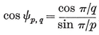 [image]
But he used his geometrical knowledge of gp,q,r in the various particular cases, and did not attempt to evaluate the integral directly.
[]
¶ CHAPTER VIII
TRUNCATION
WE have described three families of regular polytopes : the simplexes an (viz., the triangle, tetrahedron, etc.), the cross polytopes βn (the square, octahedron, etc.), the measure polytopes γn (the square, cube, etc.) ; and the one family of cubic honeycombs δn.[image]
{3, 4, 3}, {3, 3, 5},
and the four-dimensional honeycombs
{3, 3, 4, 3}, {3, 4, 3, 3}.
[image]{.image .placeholder original-image-src=“content/images/00114” original-image-title=“” width=“0in” height=“0in”}p, q, . . . , w}, in terms of a new symbol (j, k[image]
[image]{.image .placeholder original-image-src=“content/images/00114” original-image-title=“” width=“0in” height=“0in”} The simple truncations of the general regular polytope. The actual vertex figures of a regular polygon {p} are the sides of another {p} which we may call a truncation of the first (as it is derived from the first by cutting off all the corners). Its vertices are the mid-points of the sides of the first ; in fact, the two {p}‘s are reciprocal with respect to the in-circle of the first, which is the circum-circle of the second. Somewhat analogously, the vertex figures and truncated faces of a regular polyhedron or tessellation {p, q p, q
p, q q}’s and two {p}’s, arranged alternately.
Again, the N0 vertex figures and N3 truncated cells of a regular polytope or honeycomb {p, q, r} are the cells, {q, r
[image]
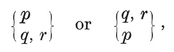
which has N1 vertices, the mid-points of the edges of {p, q, r[image]{.image .placeholder original-image-src=“content/images/00114” original-image-title=“” width=“0in” height=“0in”}p} of {p, q, r} ; it is thus an edge of one vertex figure {q, r}, and also a vertex figure of one face {p}. But such a {p} is the common face of two cells {p, q} of [p, q, r q, r
q, r p} as interfaces. (Sections of these are indicated in Fig. 8.1A.)
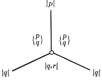
[image]{.image .placeholder original-image-src=“content/images/00114” original-image-title=“” width=“0in” height=“0in”}p, q, r}, are the centres of the {r}’s of a reciprocal {r, q, p}, it is natural to let
[image]
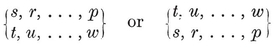
denote the polytope (or honeycomb) whose vertices are the centres of the {p, … , r}’s of {p, … , r, s, t, u, . . . , w}, or the centres of the {w, . . . , u}’s of {w, . . . , u, t, s, r, . . . , p}. Such “truncations” of a given regular figure arise at special stages of a continuous process which, in the finite case, may be described as follows.
When a regular polytope {p, q, . . . , w} is reciprocated with respect to a concentric sphere of radius 0R, its vertices are the centres of the cells of the reciprocal polytope {w, . . . , q, p}. For any greater radius of reciprocation, the former polytope is entirely interior to the latter. Let the radius gradually diminish. Then the sphere shrinks, and the reciprocal polytope shrinks too. As soon as the radius is less than 0R, the bounding hyperplanes of {w, . . . , p} cut off the corners of {p, . . . , w}. What is left, namely the common part of the content of the two reciprocal polytopes, is (in a more general sense) a truncation of either.
In gradually diminishing, the radius of reciprocation takes (at certain stages) the values 0R, 1R, . . . , *n*−1R. In the last case, the vertices of {w, . . . , p} are at the centres of the cells of {p, . . . , w} ; so here, and for any smaller values, the truncation is just {w, . . . , p} itself. When the radius of reciprocation is kR (0<k<n−1), the sphere touches the Π*k’s of {p, . . . , w} and the Πn−k−*1’s of {w, . . . , p}, or, let us say,
the {p, . . . , r}’s of {p, . . . , w) and the {w, . . . , u}’s of {w, . . . , p}.
At a point of contact, the {p, . . . , r} and {w, . . . , u[image]{.image .placeholder original-image-src=“content/images/00114” original-image-title=“” width=“0in” height=“0in”}0R, 1R, 2R, . . . , *n*−3R, *n*−2R *n*−1R determine the polytopes
[image]
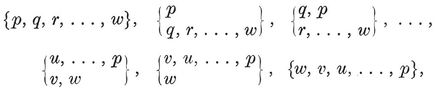
whose vertices are the centres of elements Π0, Π1 Π2, . . . , Π*n*−3′ Π*n*−2′ Π*n*−1 of the original polytope.
While the radius of reciprocation is diminishing from the value 0R, the polytope {p, q, . . . , w} has all its corners cut off and replaced by new cells {q, . . . , w}. These increase in size until the radius reaches the value 1R, when the cells {q, . . . , w p, q, . . . , w
 p, q, . . . , v
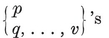
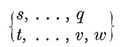
and
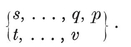
In terms of properties of {p, . . . , w}, there are N0 cells of the former kind, and Nn−1 of the latter.
[image]{.image .placeholder original-image-src=“content/images/00114” original-image-title=“” width=“0in” height=“0in”}s, r, … , p} and {t, u, … , w}, which have a common edge, { }. The plane faces are {s} and {t}; the solid faces are {s, r}, t, u}; and so on.
Besides these simple truncations there are some interesting intermediate truncations ; e.g., in the two-dimensional case, a certain radius between 0R and 1R determines {2p} as a truncation of {p}. But the investigation of such figures would take us too far afield.
[image]{.image .placeholder original-image-src=“content/images/00114” original-image-title=“” width=“0in” height=“0in”}β4 β4
β4 Fig. 8.1A with p=q=3, r=4.) Hence this truncation of β4 is regular :
[image]
If any confirmation were needed, we might observe that its vertex figure, being a convex polyhedron with square faces, can only be a cube.
Thus the regular polytope {3, 4, 3} (Fig. 8.2A) has 24 octahedral cells. Being self-reciprocal (as its Schläfli symbol is palindromic), it has also 24 vertices, namely the centres of the edges of β4[image]
N0 = 24, N1,= 96, N2 = 96, N3 = 24.
[image]
[image]
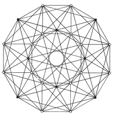
FIG. 8.2B β4 and γ4
The construction exhibits [3, 3, 4] as a subgroup in [3, 4, 3]. Since g3,3,4 = 24[image]{.image .placeholder original-image-src=“content/images/00114” original-image-title=“” width=“0in” height=“0in”}β4’s and consequently lie in the bounding hyperplanes of three γ4’S. Whichever set of 8 octahedra we pick out, the remaining 16 lie in the bounding hyperplanes of that β4. Hence the cells of β4 lie in the bounding hyperplanes of two γ4’s, and the cells of {3, 4, 3} lie in the bounding hyperplanes of three γ4’s. Reciprocally, the vertices of γ4 belong to two β4’s, and the vertices of {3, 4, 3} belong to three β4’s.
Again, the bounding hyperplanes of {3, 4, 3} belong (in three ways) to one γ4 and one β4; reciprocally, the vertices of {3, 4, 3} belong (in three ways) to one β4 and one γ4. In the latter case (Fig. 8.2B) the 32 edges of the γ4 occur among the 96 edges of {3, 4, 3} ; the remaining 64 fall into 8 sets of 8, joining each vertex of the β4 to the vertices of the corresponding cell of the γ4. Thus the 24 cells of {3, 4, 3} are dipyramids based on the 24 squares of the γ4. (Their centres are the mid-points of the 24 edges of the β4.)
We mentioned, in § 2·7, a construction for the rhombic dodecahedron from two equal cubes. We now have an analogous construction for {3, 4, 3} from two equal hyper-cubes. Cut one of the γ4’s into 8 cubic pyramids based on the 8 cells, with their common apex at the centre. Place these pyramids on the respective cells of the other γ4. The resulting polytope is {3, 4, 3}. We shall refer to this as Gosset’s construction for {3, 4, 3}. It is related to Cesàro’s by reciprocation : Cesàro cuts pyramids from the corners of β4, while Gosset erects pyramids on the cells of γ4.
Incidentally, we have found four regular compounds. By a natural extension of the notation defined in § 3·6, these are
γ4[2 β4], [2 γ4]β4,
{3, 4, 3}[3 β4]2{3, 4, 3}, 2 [3 γ4] {3, 4, 3}.
Other compounds will be found in § 14·3.
8·3. Coherent indexing. We saw in § 3·7 how the edges of an octahedron can be “ coherently indexed ” in such a way that the four edges at any vertex are directed alternately towards and away from the vertex. The sides of each face are directed so as to proceed cyclically round the face, and alternate faces acquire opposite orientations. In other words, the octahedron has four clockwise and four counterclockwise faces (as viewed from outside).
If the polytope {3, 4, 3} can be built up from 24 such octahedra, so that each triangle is a clockwise face of one octahedron and a counterclockwise face of another, then we shall have a coherent indexing for all the 96 edges of {3, 4, 3}. But it is not obvious that such “ building up ” can be done consistently. We therefore make a deeper investigation, as follows.
Let us reciprocate a coherently indexed octahedron, and make the convention that each edge of the cube shall be indexed so as to cross the corresponding edge of the octahedron from left to right (say). The consequent indexing of the edges of the cube is naturally not “ coherent,” but each edge is directed away from a vertex of one of the two inscribed tetrahedra and towards a vertex of the other. The same kind of “ alternate ” indexing can be applied to the edges of γ4, by means of its two inscribed β4’s.
Now consider Gosset’s construction, where {3, 4, 3} is derived from γ4 by adding eight cubic pyramids. The “ alternate ” indexing of the γ4, and consequently of each of the eight cubes, enables us to make a coherent indexing of the cubic pyramids, and consequently of the whole {3, 4, 3}.
The general statement, of which this is a particular case, is that the edges of a polytope or honeycomb {p, q, . . . , w} can be coherently indexed if, and only if, q is even.
8·4. The snub {3, 4, 3}. In § 8·2 we derived {3, 4, 3} from {3, 3, 4}. In § 8·5 we shall derive {3, 3, 5} from {3, 4, 3}, not directly but with the aid of a kind of modified truncation which we proceed to describe.
 Fig. 8.1A with p=3, q=4, r
Instead of bisecting the edges of {3, 4, 3}, let us now divide them in any ratio a : b α≥b. In the limiting case when a/b approaches 1, the irregular icosahedron becomes a cuboctahedron (Fig. 8.4A) with one diagonal drawn in each square face. But each square face belongs also to a cube. Hence in this case all the cubes likewise have one diagonal drawn in each face. The question arises, Which diagonal ? The only way to preserve tetrahedral symmetry is to take those diagonals which form the edges of a regular tetrahedron inscribed in the cube (Fig. 8.4B). The cube is then divided into five tetrahedra : the regular one, and four low pyramids. When α/b increases, the regular tetrahedron remains regular ; but the pyramids grow taller, and there is no reason to expect them to remain in the same 3-space.

When α/b
s{3, 4, 3},
having 96 vertices, 288+144 edges, 96+96+288 triangular faces, 24+96 tetrahedra, and 24 icosahedra. One type of edge is surrounded by one tetrahedron and two icosahedra, the other by three tetrahedra and one icosahedron.
8·5. Gosset’s construction for {3, 3, 5}. Since the circum-radius of an icosahedron is less than its edge-length, we can construct, in four dimensions, a pyramid with an icosahedron for base and twenty regular tetrahedra for its remaining cells. Let us place such a pyramid on each icosahedron of s{3, 4, 3}. The effect is to replace each icosahedron by a cluster of twenty tetrahedra, involving one new vertex, twelve new edges, and thirty new triangles. Thus we obtain a polytope with 96+24 vertices, 288+144+288 edges, 96+96+288+720 triangular faces, and 24+96+480 tetrahedral cells. For the purpose of counting the number of cells that surround an edge, each icosahedron of s{3, 4, 3} counts for two tetrahedra. Thus an edge of any of the three types is surrounded by just five tetrahedra. This, therefore, is the regular polytope
{3 3, 5},
and we have found that N0=120, N1=720, N2=1200, N3=600. (See Plates IV and VII.)
It follows by reciprocation that the remaining four-dimensional polytope {5, 3, 3} has 600 vertices, 1200 edges, 720 pentagonal faces, and 120 dodecahedral cells. (Plates V and VIII.)
By 7·62, the symmetry group [3, 3, 5] (of either of these two reciprocal polytopes) is of order
8·51
The construction indicates that a certain subgroup of index 2 in [3, 4, 3] is a subgroup of index 25 in [3, 3, 5]. In fact, the vertices of {3, 3, 5}, each taken 5 times, are the vertices of 25 {3, 4, 3}’s. (See Table VI(iii) on page 303.)
We have now established the existence of all the polytopes 7·81. As for the honeycombs 7·84, we begin with δ5
and the centres of its cells are the vertices of the reciprocal honeycomb
{3, 3, 4, 3}.
Thus four-dimensional space can be filled with β4’s, or with {3, 4, 3}’s, just as well as with γ4’s. It follows, incidentally, that the dihedral angle of either β4 or {3, 4, 3} is exactly 2π/3.
Another case of a regular “ truncation ” is
8·6. Partial truncation, or alternation. We saw, in §§ 3·6, 4·2, 4·7, and 8·2, that it is possible to select alternate vertices of {4, 3} or {4, 4} or {6, 3} or {4, 3, 4} or {4, 3, 3} in such a way that every edge has one end selected and one end rejected. Since this can also be done to any even polygon, it is natural to expect that it can be done to every polytope or honeycomb {p, q, r, … , w} with p even. (It obviously cannot be done when p[image]{.image .placeholder original-image-src=“content/images/00114” original-image-title=“” width=“0in” height=“0in”}whenever every face Π2 has an even number of sides. The details are as follows.
A polytope or honeycomb is said to be simply-connected if it is topologically equivalent to a “ map ” drawn (without any overlapping of cells) on a sphere or a flat space, respectively. (This is certainly the case for all the figures so far considered, except those in Chapter VI. The honeycombs cover a flat space by definition, and the polytopes can be projected onto concentric spheres without altering their topology.) Hence a circuit of edges can be shrunk to a point without leaving the manifold (i.e., without leaving the “ surface ” of the polytope). In other words, such a circuit is (generally in many different ways) the boundary of a two-dimensional region or “ 2-chain,” consisting of a number of Π2’s fitting together in such a way as to be topologically equivalent to a circle with its interior, or to the curved surface of an ordinary hemisphere. If the circuit consists of N edges, we can transform the 2-chain into a complete topological polyhedron (or two-dimensional map) by adding one N[image]{.image .placeholder original-image-src=“content/images/00114” original-image-title=“” width=“0in” height=“0in”}2 has an even number of sides, the number N must be even too. Finally, we select those vertices of the polytope or honeycomb which can be reached from a given vertex by proceeding along an even number of edges. Since every circuit is even, this can never give an ambiguous result ; we shall have selected just half the vertices.
If Π*n={p, q, r, . . . , w}, where p is even, let us use the symbol hΠn* to denote the polytope or honeycomb whose vertices are alternate vertices of Πn ; e.g.,
(The “h” may be regarded as the initial for either “half” or “ hemi.”)
These instances make it clear that hΠ*n* is a partial truncation in the sense that, when Π*n* is a polytope, the rejected corners are cut off by hyperplanes parallel to those of the corresponding vertex figures. In fact, h{p, q, . . . , v, w}, with p even, has
N00 cells {q, . . . , v, w},
and
Nn−1 elements h{p, q, … , v}.
The last are cells, except in the case of h{p} or h{4, q}. Since h{ } is a single point, while h{4} is a digon, the partially truncated sides of {p} are not sides but vertices of h{p}, and the partially truncated faces of {4, q} are not faces but edges of h{4, q}.
Since
[image]
while in higher space the cells of h{4, q, . . . , v, w} are {q, . . . , v, w) and h{4, q, … , v}, an appropriate extension of the Schläfli symbol is
For, we can now assert that the cells of this polytope or honeycomb are
{q, r, . . . , v, w
This notation covers every case except h{p}={p/2} and h{6, 3}={3, 6}. But it is not so far-reaching as it looks, since actually q=r= . . . =v=3, and we have only
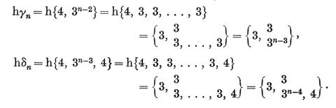
The polytope hγ*n* is regular when n=1, 2, 3, 4 :
hγ1 = α0, hγ2 = α1, hγ3 = α3, hγ4 = β4.
The honeycomb hδ*n* is regular when n=2, 3, 5 :
hδ2 = δ2, hδ3 = δ3, hδ5 = {3, 3, 4, 3}.
(The regularity of hδ5 follows from the fact that its cells, β4 and hγ4, are alike.)
The possibility of selecting alternate vertices of δn+1 gives, by reciprocation, the possibility of selecting alternate cells of δ*n*+1, say white and black cells. In other words, the chess-board has an n-dimensional analogue. When n=4, take a white γ4, and place on each of its eight cells a cubic pyramid consisting of one-eighth part of the neighbouring black γ4. We thus obtain a {3, 4, 3} (by Gosset’s construction, page 150). Such {3, 4, 3}’s, derived from all the white γ4’s, will exactly fill the four-dimensional space, coming together in sets of eight at the centres of the black γ4’s, as well as at the vertices of the δ5. We thus obtain {3, 4, 3, 3}. (The analogous procedure in three dimensions leads to the honeycomb of rhombic dodecahedra, which is the reciprocal of hδ4
[image]{.image .placeholder original-image-src=“content/images/00114” original-image-title=“” width=“0in” height=“0in”} Much of the above discussion can be simplified by the use of coordinates. If we take the vertices of β4 to be the permutations of
[image]
we immediately deduce the mid-points of its edges, which are the vertices of {3, 4, 3}, as being the permutations of
[image]
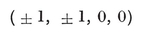
[image]
x1=±1, x2=±1, x3=±1, x4=±1, and ±x1±x2±x3±x4=2.
Hence the vertices of the reciprocal {3, 4, 3} (with respect to the sphere x12+x22+x32+x42[image]
[image]
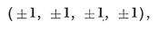
which we recognize as the vertices of β4 and γ4 (Fig. 8.2B).
[image]{.image .placeholder original-image-src=“content/images/00114” original-image-title=“” width=“0in” height=“0in”}a : b (where α+b=1) by points whose coordinates are the even permutations of
(±1, ± α, ± b, 0).
Putting α=τ−1, b=τ−2, and multiplying through by τ, we obtain the vertices of s{3, 4, 3} as even permutations of
8.74
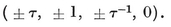
[image]{.image .placeholder original-image-src=“content/images/00114” original-image-title=“” width=“0in” height=“0in”}τ, 1, ±τ−1, 0), namely 2τ−1.
Locating the centres of the tetrahedra of various types, and multiplying through by 4τ−2, we obtain the 600 vertices of the reciprocal {5, 3, 3} (of edge 2τ−2) as the permutations of

along with the even permutations of
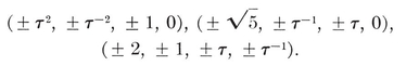
The simplest coordinates for the n+1 vertices of the regular simplex an
8.75

i.e., 1 and n 0’s, in the hyperplane Σx=1 of (n+1)-dimensional space. An element α*j* is given by restricting the permutations so as to allow the 1 to occupy any one of j+1 definite positions. Hence the centre of a typical α*j* (after multiplying through by j+1) is
(1*j*+1, 0*n-j*).
 *j*+*k*} has for vertices the permutations of
[image]

Similarly, the vertices of the cross polytope βn are the permutations of
[image]

[image]
 j+1 odd and k+1 even coordinates. In particular, the vertices of {3, 4, 3, 3} have two odd and two even coordinates.
The 2*n* points (±1*n) are, of course, the vertices of the measure polytope γn (of edge 2). From these we pick out the 2*n*−1 vertices of the “ half measure polytope ” hγn* (of edge 2√2) by allowing only even (or only odd) numbers of negative signs. This rule is justified by the fact that every edge of yn joins two points which differ by unity in their number of negative signs.
The cubic honeycomb δ*n*+1 (of edge 1) is formed by all the points with n integral coordinates. From these, we pick out the vertices of hδn+1 (of edge √2) by restricting the coordinates to have an even (or odd) sum. For, an edge of δ*n*+1 joins two points whose coordinates differ by unity in just one place. In particular, the vertices of {3, 3, 4, 3}=hδ5 can be taken to have four coordinates with an even sum, in every possible arrangement.
[image]{.image .placeholder original-image-src=“content/images/00114” original-image-title=“” width=“0in” height=“0in”} The circum-radius 0R[image]
 n of edge 2l,
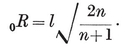
Alternatively, we may use the general formula
[image]
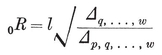
[image]
The other radii jR can be deduced from the fact that the triangle O0 O*j* O*n* is right-angled at O*j. (See § 7.9.) We merely have to subtract the squared circum-radius of a j-dimensional element from the squared circum-radius of the whole polytope ; e.g., for an*,
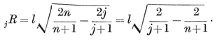
The angular properties φ=O0 O*n* O1, χ = O0 O*n* O*n*−1, ψ=O*n*−2 O*n* O*n*−1 are then given by
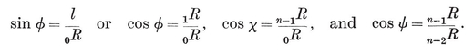
From the last of these we deduce the dihedral angle π–2ψ.
If we know the content Cp, . . . , v of a cell, and the number of cells, we obtain the surface-analogue as
S = Nn−1 Cp, . . . , v.
By dissecting the polytope into Nn−1 pyramids with their common apex at the centre, we obtain the whole content (or volume-analogue) as
8·82
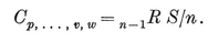
These formulae enable us to prove by induction that the contents of αn, βn, γn are respectively
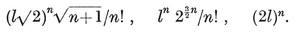
(Of course the last of these results is obvious from first principles. In the case of βn, the cell is α*n*−1, so induction is not needed there. Other special cases can be seen in Table I, on page 293.)
If general formulae are desired (in terms of p, q, … , w), the best procedure is to define n numbers
(− 1, 1), (0, 2), (1, 3), . . . , (n − 2, n)
so as to satisfy the relations
8·83
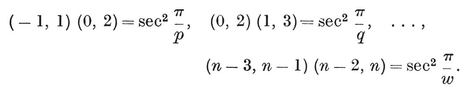
Further numbers (j, k) are then defined by (j, j)=0, (j, j+1)=1,
[image]
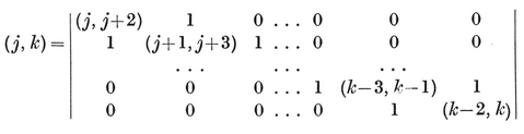
and (k, j)=−(j, k) whence109
[image]
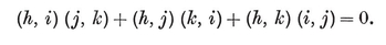
It follows that (0, k)/(-1, k) is the kth convergent of the continued fraction
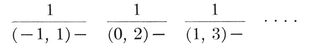
One of the n numbers (-1, 1), … , (*n-*2, n[image]{.image .placeholder original-image-src=“content/images/00114” original-image-title=“” width=“0in” height=“0in”}j, k)’s in a triangular table
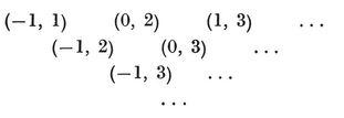
by means of the recurrence formula
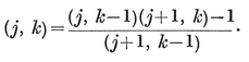
For instance, when n=3 we might take (0, 2)=1 and deduce
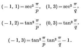
PLATE IV
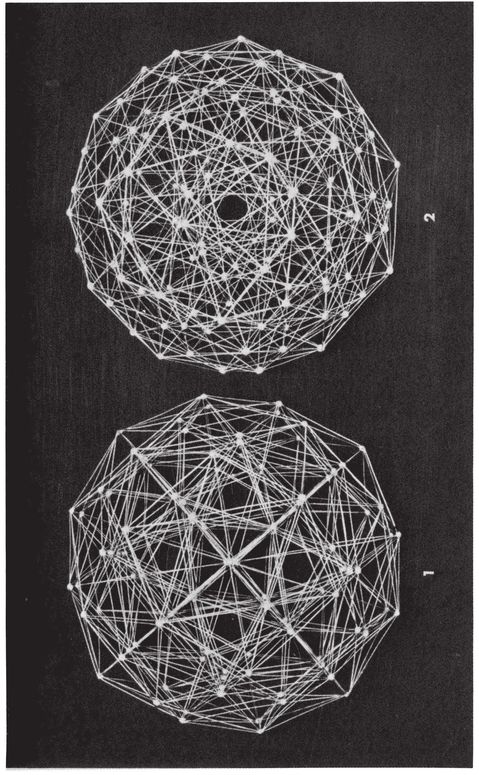
TWO PROJECTIONS OF
Dividing the kth row and column of the determinant
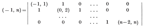

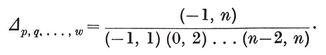
Similarly,
[image]
[image]
[image]
[image]
Since
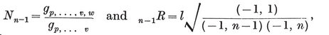
[image]
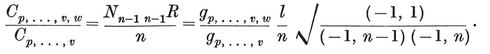
There are analogous expressions for Cp, . . . , u, v/Cp, . . . , u, etc., ending with
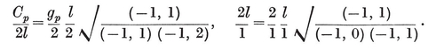
Multiplying these n equations together, we deduce
[image]
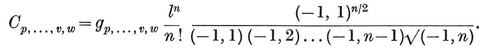
We have seen that one of the numbers (-1, 1), (0, 2), … , (*n-*2, n) can be chosen as we please. It happens that the best choice is (0, 2)=2, whenever n>3. Then the values for all the numbers (j, k) are as follows :
¶ –
In the last case, a concise summary is (−1, k)=1−kτ−3 (k≥0).
8·9. Historical remarks. In § 8·2 we obtained {3, 4, 3} by taking, as vertices, the mid-points of the edges of the cross polytope β4. We have ascribed this construction to Ernesto Cesàro (1, p. 65) because, although Schläfli must have understood it, he did not actually say so. The general “ curtail ”
8·91

 golden section ; this was pointed out by Mrs. Stott in 1931.110
 r} ; and the vertex figure of s{3, 4, 3} is a solid bounded by five triangles and three pentagons (Fig. 8.9A), which may be derived from an icosahedron (the vertex figure of (3, 3, 5}) by truncating three non-adjacent corners, i.e., by cutting off three pentagonal pyramids, just as s{3, 4, 3} itself can be derived from {3, 3, 5} by cutting off 24 icosahedral pyramids. The still more remarkable last part of Gosset’s essay is concerned with the polytopes k21 which we shall construct (in a quite different manner) in § 11-8.
The general theory in § 8·6 is new, but the idea of partial truncation was suggested by Mrs. Stott (2, p. 15) and the sig-nificant
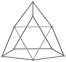
The vertex figure of s
cases hγn, hδn were discussed analytically by Schoute (10, pp. 73, 90). The identity
hδ5 =
may be said to have been anticipated by Gosset in his (reciprocal) remark that the cells of {3, 4, 3, 3} are concentric with alternate cells of δ5 ; this enabled him to construct all the regular polytopes and honeycombs without using any “ deeper ” truncation than 8·91.
The general process of truncation (§ 8·1) is a special combination of Mrs. Stott’s two processes of expansion and contraction,111 k’s of Π*n* is cek Π*n*. But she also defined other polytopes
ei . . . ek Π*n* and cei . . . ek Π*n* (0<i< . . . <k<n)
which, unfortunately, are beyond the scope of this book.
The coordinates that we found for {3, 4, 3} in § 8·7 are due to Schläfli (4, p. 51). He also obtained coordinates for {3, 3, 5}, but with a different frame of reference (p. 121). The coordinates chosen here are due to Schoute (6, pp. 210-213), 112though he failed to observe that the points 8·74 by themselves form a semi-regular polytope.
We saw, in § 4·4, that the vertices of {4, 4} may be regarded as representing the Gaussian integers. Analogously, the vertices of {3, 3, 4, 3} (whose coordinates are either four integers or four halves of odd integers) represent Hurwitz’s integral quaternions (see Dickson 1, p. 148). The vertices of {3, 4, 3} (viz., 8·71 and 8·73, divided by 2) represent the 24 “ units ”
±1, ±i, ±j, ±k, (±1±i±j±k)/2
of that arithmetic.
It was Schläfli (4, pp. 52-56) who found the radii, angles, and content of each regular polytope, as in § 8·8 ; but he did not attempt to give a general formula for content, such as 8·87.
Thorold Gosset was born in 1869. After a largely classical schooling, he went up to Pembroke College, Cambridge, in 1888. He was called to the Bar in 1895, and took a law degree the following year. Then, having no clients, he amused himself by trying to find out what regular figures might exist in n dimensions. After rediscovering all of them, he proceeded to enumerate the “ semi-regular ” figures. He recorded the results in the above-mentioned essay, which he sent to Glaisher in 1897. Glaisher showed it to Whitehead and Burnside. It is tempting to speculate on the possibility that some of its ideas, unconsciously assimilated, bore fruit in Burnside’s later work. This, however, is unlikely ; for Burnside declared (in a letter to Glaisher, dated 1899) that he never found time to read more than the first half. “ The author’s method, a sort of geometrical intuition ” did not appeal to him, and the idea of regarding an (n−1)-dimensional honeycomb as a degenerate n-dimensional polytope seemed “ fanciful.” He thus failed to appreciate the new discoveries, and Glaisher was content to publish the barest outline. That published statement remained unnoticed until after its results had been rediscovered by Elte and myself. As he was a modest man, Gosset let the subject drop, and pursued his career as a lawyer. He died in 1962 at the age of 93.
[]
¶ CHAPTER IX
POINCARÉ’S PROOF OF EULER’S FORMULA
THE discoverer and earliest rediscoverers of the regular polytopes (viz., Schläfli, Stringham, Forchhammer, Rudel, and Hoppe) all observed that the total number of even-dimensional elements and the total number of odd-dimensional elements are either equal (as in the case of a polygon) or differ by 2 (as in the case of a convex polyhedron). Schläfli (4, p. 20), like most of the others, attempted a general proof; but the dependence on simple-connectivity was not properly appreciated until 1893, when Poincaré wrote a short note on the subject, which he expanded six years later.113
This, like the last half of Chapter I, belongs to the realm of topology (or analysis situs). Incidentally, it seems odd that topologists have never adopted the word “ polytope.” They continually use “simplex.” The antithesis, “complex,” means a collection of polytopes meeting one another at any kind of element ; e.g., a one-dimensional complex is a graph.
9·1. Euler’s Formula as generalized by Schläfli. Consider the following sequence of propositions.
¶ –
(We proved this in § 4·8.)
Schläfli exhibited these as special cases of the formula
N0−N1+N2− . . . +(−1)*n*−1Nn−1=1−(−1)n
or
9·11 N*0−N1+N2−* . . .Nn*−1*±Nn=1
or
N−1−N0+N1− . . . ±NnNn=0,
which holds for any simply-connected polytope Π*n.*
This is verified for the regular polytopes αn, βn, γn by setting X = −1 in 7·41. As an instance where the polytope is not regular, we may take the s{3, 4, 3} of § 8·4, for which
N0 = 96, N1 = 432, N2 = 480, N3 = 144,
or the hγ5 of § 8·6, for which
N0 = 16*, N*1 = 80, N2 = 160, N3 = 120, N4 = 26.
But the general case is not so easy. The usual proof by induction (e.g., Somerville 3, p. 147) is the natural extension of Euler’s own proof of 1·61, and involves the same kind of unjustified assumption about the manner in which a polytope may be gradually taken apart or built up. The following procedure is an attenuated version of Poincaré’s deduction of the analogous formula for a circuit (i.e., a generalized polytope which may be multiply-connected).
9·2. Incidence matrices. It must be emphasized that 9·11 is a theorem of topology, which is more general than ordinary geometry in that it is not concerned with measurement, nor even with straightness. The polytope Π*n* may be distorted (by bending and stretching, as if it were made of rubber) without changing the essential relationship of its vertices Π0, edges Π1, plane faces Π2, solid faces Π3, . . . , and cells Π*n*−1. In fact, its topological nature is determined when we know which Π*k*−1’s are cells of each Π*k* (for k=1, 2, … , n). This information is expressed concisely in terms of incidence numbers
Let the various Π*k*’s (for each k
 k these numbers form an incidence matrix (or rectangular table) of Nk−1 rows and Nk columns. The ith row shows which Π*k
 jth column shows which Π*k*−1*n*−1’s are cells of the whole polytope Πn*
9·21
Dually, as in § 7·4, we regard all the elements as having a common “null” element Π−1 ; in other words, we make the convention
9·22

Consider, for example, a tetrahedron ABCD (n=3) with edges AD, BD, CD, BC, AC, AB, and faces BCD, ACD, ABD, ABC. Here the η’s are the entries in the following four tables :
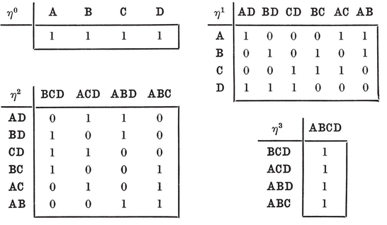
For an obvious reason, we have chosen a very simple example. The incidence matrices for {3, 3, 5} would fill a big book; and in § 11·8 we shall have occasion to describe an eight-dimensional polytope (called 421) whose incidence matrices would fill about a million books.
9·3. The algebra of k-chains. A k-chain is defined to be any selection of Π*k*’s (for a definite k), considered as the sum *k*+1 is a special k-chain which we call the boundary of the Π*k*+1. The sum of two k-chains is defined as consisting of the distinct elements of both, with any common elements omitted. Thus a k-chain is a formal sum

where each xj=0 or 1 ; and the sum of two k-chains is
9·31
with the coefficients reduced modulo 2. In other words, the coefficients are not ordinary numbers but residue-classes,114 “ 0 ” and “ 1” meaning “even” and “odd.” These combine according to the finite arithmetic
9·32

This convention enables us to define the boundary of a k-chain as the sum of the boundaries of its Π*k’s. For, if the k-chain contains two Πk*’s which are juxtaposed to the extent of having a common Π*k*−1, this is naturally no part of the boundary of the k-chain. In particular, the boundary of a Π*k*+1 is a k-chain whose bounding (k−1)-chain vanishes ; i.e., it is an unbounded k-chain, or k-circuit. So also the boundary of any (k+1)-chain is a k-circuit.
In the tetrahedron used as an example above, the boundary of the 2-chain ABC+BCD is
AB**+AC+BC+BC+BD+CD=AB+AC+BD+CD;**
and this 1-chain is a 1-circuit, as its boundary is
A+B+A+C+B+D+C+D=0.
*k*−1’s which are incident with it, namely
and the boundary of the k-chain Σxji and j). In particular, Σ xjk-circuit if
9·33
for each i. On the other hand, Σ xjbounding k-circuit if it is the boundary of some (k+1)-chain Σ yl yl (l=1, 2, . . . , Nk+1) such that
9·34
We are regarding 9·33 and 9·34 as equations whose coefficients and unknowns belong to the finite arithmetic 9·32. But we could just as well regard them as congruences, by writing “ = (mod 2) ” instead of “ =.”
The convention 9·22 implies that the 0-chain Σ xjxj=0, i.e., if the number of its points is even. In saying that the boundary of a (k+1)-chain is a k-circuit, we implied that k>0 ; but our convention makes this hold also when k=0. Conversely, any 0-circuit, consisting of (say) 2m vertices, is the boundary of a 1-chain consisting of m connected sequences of edges.
When k=n−1, 9·34 shows that the condition for Σ xj n−1)-circuit is that all the x’s be equal (to y1). The case when they all vanish is of course excluded ; hence every xj=1, and the only bounding (n
 n.
n.
9·4. Linear dependence and rank. The rule 9·31 suggests the abstract representation of the k-chain Σ xjx1, x2, . . . , xNk) whose components xjj=1, 2, . . . , Nk) form a basis, in the sense that every vector is expressible as a linear combination of these Nk. In other words, the class of k-chains can be represented as an Nk-dimensional vector space115 (over the field of residue-classes modulo 2).
The class of k-circuits constitutes a subspace of this vector space. The number of dimensions of the subspace is the number of independent k-circuits, or the number of independent solutions of the Nk−1 homogeneous linear equations 9·33 for the Nk unknown x’s.
The bounding k-circuits likewise form a subspace. Its number of dimensions, being the number of independent bounding k-circuits, is the number of independent vectors (x1, x2
As a step towards the computation of these numbers, we proceed to define “ rank.” By selecting certain rows of a matrix, and the same number of columns, we obtain a square submatrix whose determinant may or may not vanish. The number of rows (or columns) is called the order of the determinant. The rank of the matrix is defined as the largest order, say p, for which a non-vanishing determinant occurs. This p may take any value from 0 (when the matrix consists entirely of zeros) to the number of rows or columns (whichever is smaller). Since each determinant of order ρ+1 vanishes, every row (or column) can be expressed as a linear combination of p particular rows (or columns), namely of those which were selected in forming a non-vanishing determinant.
For instance, the matrices η1 and η2 on page 167 are both of rank 3.
9·5. The k-circuits. Let ρk x’s, only ρk of the Nk−1 equations are really needed ; the rest are algebraic consequences of those ρk. We thus have to solve ρk homogeneous equations for Nk unknowns. If Nk=ρk+1, there is a unique solution (not counting the trivial solution where all the x’s vanish). If Nk=ρk+1+δ, where δ>0, the equations can still be solved after arbitrary values have been assigned to δ of the x’s. In either case, the equations have Nk−ρk independent solutions. Accordingly, this is the number of independent k-circuits.
In particular, the rank of a single row of 1’s (see 9·22) is
9·51

A simple set of N0−ρ0 independent 0-circuits is
In the case of the tetrahedron, the matrix η1 provides the four equations
x1 + x5 + x6 = 0, x2 + x4 + x6 = 0, x3 + x4 + x5 = 0, x1 + x2 + x3 = 0,
of which the last can be obtained by adding the first three. These have the N1−ρ1=3 independent solutions
(0, 1, 1, 1, 0, 0), (1, 0, 1, 0, 1, 0), (1, 1, 0, 0, 0, 1),
corresponding to the 1-circuits
BD**+CD+BC,** AD**+CD+AC,** AD**+BD+AB.**
9·6. The bounding k-circuits. The equations 9·34 define vectors (x1, x2ρk+1. Accordingly, this is the number of independent bounding k-circuits.
In particular, the rank of a single column of 1’s (see 9·21) is
9·61

and the only bounding (n−1)-circuit is the boundary of Π*n* itself.
The matrix η2 on page 167 has ρ2=3 independent columns. Any three of the four columns will serve. The first three provide the 1-circuits
BD + CD + BC, AD + CD + AC, AD + BD + AB,
which bound the faces BCD, ACD, ABD of the tetrahedron.
9·7. The condition for simple-connectivity. We saw, in § 9·3, that every bounding k-chain is a k-circuit. The special property which distinguishes a simply-connected polytope Π*n* is that, conversely, every k-circuit is the boundary of some (k+1)-chain. (When n=3 and k=1, this resembles the statement that a closed surface is simply-connected if every closed curve drawn on it can be shrunk to evanescence.) It follows that in this case the number of indepedent k-circuits is no greater than the number of independent bounding k-circuits : Nk − ρk = ρk+1. Hence
9·71
From this we immediately deduce
which is 9·11.
This completes the proof. The cancellation of p’s is essentially due to the fact that the rank of a matrix is both the number of independent rows and also the number of independent columns.
9·8. The analogous formula for a honeycomb. For application in § 11·8 we need the extension of 9·11 to honeycombs. This extension cannot be proved by pure topology, because it depends on the Euclidean metric. (It does not hold in hyperbolic space of an even number of dimensions, although such a space is topologically indistinguishable from Euclidean.) As in §§ 4·1 and 4·8, we consider a finite portion of an n-dimensional honeycomb, consisting of Nn−1 cells Πn, and Nj of each lower element Π*j*. By regarding the whole exterior region as one further cell, we obtain a topological Π*n*+1. Hence, by 9·11,
N0 − N1 + N2 −… + (−1)nNn = 1−(−1)*n*+1.
If the chosen portion can be enlarged in such a way that the increasing numbers Nj tend to become proportional to definite numbers νj, we conclude that
9·81
ν0 − ν1 + ν2 − . . . +(−1)nνn = 0.
In particular, if the honeycomb has a symmetry group, transitive on its vertices (so that N0*j* is the same at all vertices), then we can apply 1·81 to the topological Π*n*+1, obtaining
j’s at a peripheral vertex of the chosen portion. Since the honeycomb is Euclidean, the number of peripheral vertices is of a lower order of magnitude than the number of internal vertices. Thus ΣNj0/N0 tends to the fixed value N0*j*j, Nj/N0 *j/*ν0. Hence 9·81 is valid in this case (which is just where we shall need it).
9·9. Polytopes which do not satisfy Euler’s Formula.
N0 − N1 + N2 = 12 − 30 + 12 = − 6.
However, Schläfli (4, p. 86) has himself provided a suggestion for properly modifying 9·11 (as Cayley modified 1·61 in 6·42). In fact, the term Nk has to be replaced by Σdd′, where d is the density of a Π*k, and d’ is that of the angular figure formed by the higher elements incident with the same Πk* (i.e., d′ is the density of the “ (k+1)th vertex figure ”).
[]
¶ CHAPTER X
FORMS, VECTORS, AND COORDINATES
THIS chapter is a collection of various results in algebra (§§ 10·1-10·3) and analytical geometry (§§ 10·4-10·8). Most of them are familiar, and the rest are closely related to known theorems. They are included here partly for their intrinsic interest, but chiefly for the sake of their applications to the theory of reflection groups, which will be developed in Chapters XI and XII. The algebraical part is mainly concerned with quadratic forms none of whose “ product ” terms have positive coefficients, especially with the condition for such a form to be incapable of taking a negative value. In the geometrical part we see how the position of a point, in n-dimensional Euclidean space, is determined by its distances from n hyperplanes (inclined to one another at given angles).
10·1. Real quadratic forms. A homogeneous polynomial of the second degree in n variables x1, . . . , xn is called a quadratic form. We shall deal only with the case where the coefficients and variables are real numbers. There are “ square ” terms such as a11 x12 ; and “ product ” terms such as 2a12 x1 x2, which we shall write as (a12+a21)x1 x2. The whole form is expressible as a double sum
10·11
where aik = akia.
A quadratic form is said to be positive definite if it is positive for all values of the variables except (0, … , 0), and to be positive semidefinite if it is never negative but vanishes for some values not all zero. It is said to be indefinite if it is positive for some values and negative for others. Thus for n=2, x12+x22 is definite, (x1−x2)2 is semidefinite, and x12−x22 is indefinite.
Let Aik denote the cofactor of aik in the determinant
a = det(aik).
Then we know that116
10·12
where the “ Kronecker delta ” δjk means 1 or 0 according as j=k or j≠k. (When j=k, 10·12 is the ordinary expansion of a by means of its kth column. When j≠k, it is the analogous expansion of a determinant with two identical columns.)
The first of the following theorems is very well known :
10·13. The determinant of a positive definite form is positive.
PROOF. This is trivial when n=1. So we use induction, and assume the result for every positive definite form in n−1 variables, such as that derived from the given positive definite form 10·11 by setting xk=0 ; i.e., we assume that Akk>0. Being positive definite, 10·11 must take a positive value when xi=Aik, in which case, by 10·12,
0<ΣΣaij xi xj = Σaδjk xj=axk = aAkk.
Hence a>0.
10·14. If a positive semidefinite form ΣΣaik xi xk vanishes for xi = zi (i = 1,. . . , n), then
Σ zi aik = 0 (k = 1, . . . , n).
PROOF. The form, being positive semidefinite, is positive or zero for all values of the x’s ; in particular, when xi = yi + λzi. Thus the inequality
0 ≤ ΣΣ aik (yi + λzi)(yk + λzk) = ΣΣ aik yi yk + 2λ ΣΣ aik zi yk
must hold for arbitrary values of λ and the y’s. But this is only possible if the coefficient of λ vanishes, which means that, for arbitrary values of the y’s,
Σ (Σ aik zi)yk = 0.
[image]
It follows that the values of (x1, . . . , xn[image]
[image]
These sets of values constitute a vector space of n−ρ dimensions, where ρa. This number n−ρ is sometimes called the nullity of the form.
In particular, if n−ρ=1, there is a solution (z1, . . . , zn) such that every solution is a multiple of this, viz., (λz1, . . . , λzn).
We need one more definition, in preparation for the important theorem 10·22. A form is said to be disconnected (German zerleg-bar ) if it is a sum of two forms involving separate sets of variables ; if not, it is said to be connected : e.g., x12+x22 is disconnected, but x12−x1 x2+x22 is connected.
10·2. Forms with non-positive product terms. We shall be specially concerned with those quadratic forms in which aik≤0 whenever i≠k. For brevity, let us call them a-forms.
10·21. If a positive semidefinite a-form vanishes for x*i=zi,* it also vanishes for xi = zi.
PROOF. The expressions ΣΣ aik zi zk and ΣΣ aik zi zk differ only in those terms for which zi zk <0. But for such terms aik ≤0. Hence
0 ≤ ΣΣ aik zi zk ≤ ΣΣ aik zi zk = 0,
and we can put “ = ” in place of “ ≤.”
10·22. Every positive semidefinite connected a-form is of nullity 1.
PROOF. Let us first suppose that a given positive semidefinite a-form vanishes for xi = zi, where z1 z2 . . . *zm*≠0 (m<n) and the remaining z’s vanish. By 10·21 and 10·14, we have
Σ zi aik = 0,
and here the only non-vanishing terms are those for which i≤m. Thus
and this sum contains no positive terms. Hence aik = 0 whenever i ≤ m and k > m ; so the form is disconnected.
It follows that, if the form is connected, we must have
z1 z2 . . . *zn*≠0.
Every solution of 10·15 must be proportional to (z1, . . . , zn) ; for, any two non-proportional solutions could be combined to give a solution with one (but not all) of the x’s equal to zero. In other words, the solutions constitute a one-dimensional vector space, and the form is of nullity 1.
Since every solution of ΣΣaikxixk=0 is proportional to the positive solution (zi, . . . , zn), the x’s for which a positive semidefinite connected a-form vanishes are either all positive or all negative or all zero. The next two theorems follow at once from this remark.
10·23. For any positive semidefinite connected a-form there exist positive numbers zi such that
Σzi aik = 0 (k = 1, . . . , n),
and these are unique, apart from the obvious possibility of multiplying all by the same constant.
10·24. If we modify a positive semidefinite connected a-form by making one of the variables vanish, we obtain a positive definite form in the remaining variables.
For instance, x12 + x22 + x32 − x2x3 − x3x1 − x1x2 is semidefinite, but x12 + x22 − x1x2 is definite.
Another property which positive semidefinite connected a-forms share with positive definite forms is the following :
10·25. The square terms of a positive semidefinite connected a-form are all positive.
PROOF. For each k there is at least one non-vanishing coefficient aik (i≠k), or else the form would be disconnected with respect to the term akk xk2. Hence we must have akk>0, to balance the negative terms in Σzi aik. (See 10·23.)
On the other hand, the following property distinguishes these from definite forms :
10·26. A positive semidefinite connected a-form becomes indefinite when any one of its coefficients is decreased.
PROOF. By 10.25, the form takes the positive value a11 for (1, 0, . . . , 0), both before and after the modification. By 10·23, there are positive numbers z1, . . . , zn such that ΣΣaik zi zi=0. But if we decrease one of the aik’s we decrease this expression. Hence the modified form is capable of both positive and negative values.
PLATE V
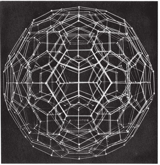
It is interesting to observe that the z’s can be expressed directly in terms of the coefficients aik :
10·27. If a positive semidefinite connected a-form vanishes for xi*=*zi, then
zi = λ√ Aii,
where Aii is the cofactor of aii in the determinant a, and λ is an arbitrary constant.
PROOF. Solving the equations 10·15 by means of determinants, we see that z1, . . . , znA. Hence
Aik = µzi zk*,*
where, by applying 10·13 and 10·24 to the case k = i, µ > 0. The desired result follows when we set µ = 1/λ2.
Incidentally, since Aik = µzi, zk, where µ, and the z’s are positive,
10·28. The adjoint of a positive semidefinite connected a-matrix has entirely positive elements.
The corresponding “adjoint form” is ΣΣAik xi xk = µ(Σzi xi)2.
10·3. A criterion for semidefiniteness. With a view to the applications we shall make in the next chapter, we wish to be able to see at a glance whether a given a-form is semidefinite. A suitable criterion is easily established by means of the following lemma :
10·31**.**

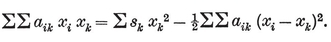
PROOF. We have
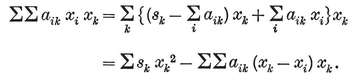
Writing the same result with i and k interchanged (in the final sum) and adding, we obtain

as desired.
Writing xi/zi instead of xi, zk sk instead of sk, and zi zk aik instead of aik, we deduce
10·32**.**
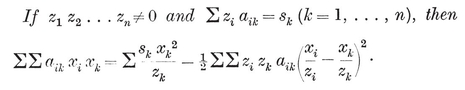
We are now ready for the criterion
10·33. If there exist positive numbers z1, . . . , zn, such that
Σzi aik = 0 (k = 1, … , n),
then the a-form ΣΣaik xi xk is positive semidefinite.
PROOF. By 10·32 with sk = 0 and zk>0 and aik ≤ 0 (i≠k), the given form is equal to a sum of squares, and so cannot be negative. But it vanishes when xk = zk. Hence it is positive semidefinite.
Combining this result with 10·23, we have
10·34. A necessary and sufficient condition for a connected a-form to be positive semidefinite is that there exist positive numbers z*1, . . . ,* zn such that Σzi aik = 0.
10·4. Covariant and contravariant bases for a vector space. The inner product (or scalar product) of two vectors x and y, in n-dimensional Euclidean space, is defined by the formula
x·y = x y cos θ,
where x and y are their magnitudes, and θ is the angle between them. In particular,
x·x = x2.
Since the space is n-dimensional, we can take n linearly independent vectors e1, e2, … , en. These span the space, in the sense that every vector x is uniquely expressible as a linear combination 117
x1e1 + x2 e2 + . . . + xnen.
The n chosen vectors ei are called a covariant basis, and the coefficients xi are called the contravariant components of the vector x. The magnitude of x is given by
10·41
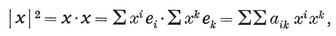
where
10·42
In particular, the magnitude of ei is ei = √aii.
The angle, θ, between x and y, is given by
10·43
In particular, non-vanishing vectors x and y are perpendicular if
ΣΣ aik xi yk = 0.
The magnitude x cannot vanish unless all the components xi vanish ; therefore the quadratic form 10·41 is positive definite, and by 10·13 its determinant a is positive.
Now, defining Aik as in 10·12, let us write aik = A*ik/a*, so that
(which means 1 or 0 according as j=k or j≠k). Consider a new set of n vectors
10·44

These again span the space, since
10·45
so we may appropriately call them the contravariant basis. A given vector x has covariant components xi, such that
x = Σxi ei.
These are related to the contravariant components by the formulae
xj = Σaij xi, xi = Σaij xj,
which are obtained by substituting 10·44 or 10·45 in the vector identity Σxi ei = Σxj ej. In this notation the inner product 10·43 is simply
10·46
So the magnitude of x is
10·47
To find a geometrical meaning for the contravariant basis, we observe that, since
each ei is perpendicular to every ej except ei. In other words, ei is perpendicular to the (n−1)-dimensional vector space spanned by n − 1 of the ej’s ; and ei is related similarly to the ej’s. More-over, the magnitude of ei is such as to make ei· ei = 1. (See Fig. 10.4A for an example with n=2. When n=3, √a e1 is the familiar outer product, or vector product, e2×e3.)
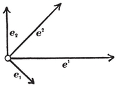
The components of x could have been defined as its inner products with the e’s; for
and similarly
x · ek = xk.
Taking x=ei in this last relation, we deduce from 10·44 that
ei · ek = aik.
(Cf. 10·42.) Thus the reciprocity between “ covariant ” and “ contravariant ” is complete.
10·5. Affine coordinates and reciprocal lattices. As soon as we have fixed an origin, 0, each vector x determines a point (x) and a hyperplane [x], namely the point whose position-vector from 0 is x, and the hyperplane through 0 perpendicular to x. If we regard the co- (or contra-) variant components of x as coordinates for (x), then the contra- (or co-) variant components are tangential coordinates for [x]. In fact, the condition for (x) and [y] to be incident, i.e., for (x) to lie in [y], is x · y=0. (Cf. 10·46.)
The distance between points (x) and (y) is
The distance between the point (x) and the hyperplane [y], measured along the perpendicular, is the projection of x in the direction of y, namely
10·51
When [y] is the coordinate hyperplane xk = 0, we have
and the distance is
10·52

The points (x) whose covariant coordinates are integers form a lattice, i.e., the set of transforms of a point by a group of translations. (See § 4·3.) The generating translations are given by the contravariant basic vectors ei. Similarly, the points whose contravariant coordinates are integers form another lattice. Crystallographers (such as Ewald 1) call these two lattices “ reciprocal.” If y1, … , yn are integers with greatest common divisor 1, the hyperplane [y] or Σyixi = 0 and the parallel hyperplane Σ*yixi* = 1 each contain infinitely many points of the first lattice, but no such point can be found between them. By 10·51, the distance between these two parallel hyperplanes (or the distance from the origin to the latter) is 1/y, i.e., the reciprocal of the distance from the origin to the point (y) which belongs to the second lattice. In other words, any “ first rational hyperplane ” of the first lattice corresponds to a point of the second lattice situated at the reciprocal distance in the normal direction. This point of the second lattice is “ visible from the origin” (i.e., it is the first lattice point in that direction) because we have supposed the coordinates yi to have no common divisor greater than 1. By interchanging “ covariant ” and “ contravariant ” we see at once that the relation between the two lattices is symmetric : each is reciprocal to the other.
The n-dimensional cubic lattice (consisting of the vertices of a δ*n*+1 of edge 1) is obviously its own reciprocal. On the other hand, the lattice of vertices of {3, 6} (§ 4·4) is reciprocal to another lattice of the same shape, rotated through a right angle about the origin (so that their vertex figures are reciprocal hexagons). Similarly in four dimensions, there are two reciprocal lattices formed by two {3, 3, 4, 3}’s with a common vertex at the origin, so placed that their vertex figures are reciprocal {3, 4, 3}’s.
The concept of reciprocal lattices must not be confused with that of reciprocal honeycombs, as defined in § 7·4; e.g., the honeycomb reciprocal to {3, 3, 4, 3} is not another {3, 3, 4, 3} out {3, 4, 3, 3} (whose vertices do not form a lattice). On the other hand, the present use of the word reciprocal is not inappropriate, as the “ visible point ” (y) is the pole of the “ first rational hyperplane” Σyi xi = 1 with respect to the unit sphere Σxi xi = 1.
10·6. The general reflection. Let (x′) be the image of (x) by reflection in the hyperplane [y]. Then x−x′ is a vector parallel to y, of magnitude twice 10·51. Thus
10·61
In particular, the reflection in the coordinate hyperplane xk=0 (where y=ek) is the transformation
10·62
If we are willing to sacrifice the reciprocity between “ covariant ” and “ contravariant,” we can take the ek’s to be unit vectors. Then akk=1, and aik is the cosine of the angle between ei and ek. By 10·52, the covariant coordinates of a point (x) are just its distances from the coordinate hyperplanes xk = 0, measured in the directions of the respectively perpendicular vectors ek. The lines along which these hyperplanes intersect (in sets of n − 1) are in the directions of the vectors ei (which, in general, are notxkek for its position vector, are the familiar “ oblique Cartesian ” coordinates, referred to axes in the directions of the unit vectors ek. The transformation 10·62 is now simply
10·63
This same result could have been obtained directly as follows. Since xk is now the distance of (x) from the hyperplane xk = 0, the reflection in that hyperplane is given by
x − x′ = 2xkek.
Taking the inner product of both sides with ei, we deduce
which is 10·63.
10·7. Normal coordinates. With reference to an n-dimensional simplex O1 O2 . . . On+1, we define the normal coordinates (x1, x2, … , xn+1) of a point to be its distances from the n+1 bounding hyperplanes, with the usual convention of sign (so that the coordinates of an interior point are all positive). These are “ trilinear ” coordinates when n=2, “ quadriplanar ” when n=3.
Let Ci denote the content of the cell opposite to Oi, and zi the reciprocal of the corresponding altitude. Then Ci/zi is n times the content of the whole simplex. So also is
C1 x1 + C2x2 + . . . + Cn+1 xn+1
for any point (x). Hence the identical relation satisfied by the n+1 x’s is
10·71
Let e1 e2, . . . , en+1 be unit vectors perpendicular to the n+1 hyperplanes, and directed inwards (towards each opposite vertex). Then
aii = ei · ei = 1,
and aik is the cosine of the angle between ei and ek ; so −aik is the cosine of the corresponding dihedral angle of the simplex. Only n of the n+1 vectors ei are linearly independent. We shall find that the relation connecting them all is
10·72
This is an important result, so we shall give two alternative proofs.
The first depends on the fact that, when a polytope is orthogonally projected onto any hyperplane, the sum of the contents of the projections of the cells is zero, provided we make a consistent convention of sign. Projecting the simplex onto a hyperplane perpendicular to a vector x, we see that the content of the projection of the ith cell is Ciei·x. Hence
(C1e1 + C2e2 + . . . + Cn+1en+1)·x = 0.
Since x is arbitrary, and the C’s are proportional to the z’s, this implies 10·72.
The second proof is more elementary but less elegant (in that it specializes one of the e’s). Let x denote the vector from O*n*+1 to any point (x1, . . . , xn, 0) on the opposite hyperplane xn+1 = 0. Then
ei · x = xi (i≤n) and en+1 · x = − 1/zn+1.
Hence, using 10·71 with xn+1 = 0,
(z1e1 + . . . + znen + zn+1en+1)· x = z1x1 + . . . + zn xn − 1 = 0.
As before, the arbitrariness of x enables us to deduce 10·72.
It follows, by taking the inner product with ek, that
10·73

(summed for the n+1 values of i).
It also follows that the quadratic form
ΣΣaik xi xk = Σ xi ei · Σ xk ek = Σ xi ei2
vanishes when xi = zi, but is never negative ; so it is positive semidefinite. Moreover, it is of nullity 1, since any n of the n+1 e’s determine a system of affine coordinates ; in fact, we obtain a positive definite form in n variables by making any one of the x’s vanish.
The reflection in xk=0 is still given by 10·63, with the range of i and k extended to n+1. For, the only possible doubt lies in the behaviour of xn+1, and 10·63 is consistent with 10·71 since, by 10·73,
10·8. The simplex determined by n+1 dependent vectors. We have seen that vectors drawn inwards (or outwards), perpendicular to the bounding hyperplanes of a simplex, satisfy the relation 10·72, where all the z’s are positive. Conversely, given n+ 1 unit vectors ei, which satisfy such a relation (with positive z’s) while e1, . . . , en are linearly independent, we can construct a corresponding simplex as follows.
Represent the n+1 vectors ei by concurrent segments M*i* I, directed towards their common point I, as in Fig. 10.8A (where n=2). Through the points M*i* so determined draw respectively perpendicular hyperplanes. These bound a simplex (with in-centre I) ; for the first n of them determine a system of affine coordinates in which the remaining hyperplane has the equation
z1x1 + . . . + znxn = 1.
10·9. Historical remarks. The only novelty about the treatment of quadratic forms in § 10·1 is the avoidance of the reduction to canonical (or diagonal) form. The proofs of 10·14, 10·21, and 10·22 are taken from Witt 1, p. 292. The first of these theorems is the natural extension of the geometrical statement that, if a cone has no real generators, its only real point is its vertex. Although § 10·2 is largely due to Witt, some properties of these “ a-forms ” (which have aik = aki ≤ 0 whenever i≠k), and of the corresponding “ a-matrices,” had already been established by other authors. Mahler (about 1939) proved that if
Σzi aik ≥ 0 (k = 1, . . . , n),
where the a’s are the coefficients of a positive definite a-form, then *zk*≥0. Du. Val (3, p. 309) deduced that the inverse of a positive definite a-matrix has no negative elements, and that a spherical simplex which has no obtuse dihedral angles has no obtuse edges either. Theorem 10·23 can be regarded as the analogue of Mahler’s result, when the a-form is semidefinite (and connected) instead of definite. Similarly 10·28 is the analogue of Du Val’s result.
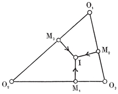
Lemma 10·32, which facilitates the proof of 10·33 in a quite spectacular manner, was discovered by W. J. R. Crosby, a research student at the University of Toronto. It shows, further, that if there exist positive numbers zi such that Σzi aik > 0, then the aa which is not necessarily symmetric. An elegant proof of that more general theorem has been given by Rohrbach (1).
[image]{.image .placeholder original-image-src=“content/images/00114” original-image-title=“” width=“0in” height=“0in”}e1, e2, e3[image]{.image .placeholder original-image-src=“content/images/00114” original-image-title=“” width=“0in” height=“0in”}118 a, b*, c*, then the Millerian face-indices h, k, l are the covariant components of a vector perpendicular to the crystal face (hkl[image]{.image .placeholder original-image-src=“content/images/00114” original-image-title=“” width=“0in” height=“0in”}119 u, v, w are the contravariant components of a vector along the zone axis, or the contravariant tangential coordinates of a plane perpendicular to all the planes of the zone [uvw]. Thus the zone axis is a diagonal of the parallelepiped formed by the vectors ue1, ve2, we3, and the condition for the face (hkl) to belong to the zone [uvw] is hu + kv + lw = 0.
[image]
[]
¶ CHAPTER XI
THE GENERALIZED KALEIDOSCOPE
[image]{.image .placeholder original-image-src=“content/images/00114” original-image-title=“” width=“0in” height=“0in”}regular[image]
[image]{.image .placeholder original-image-src=“content/images/00114” original-image-title=“” width=“0in” height=“0in”} In n-dimensional Euclidean space the reflection in a hyperplane w is the special congruent transformation that preserves every point of w and interchanges the two half-spaces into which w decomposes the whole space. In terms of rectangular Cartesian coordinates, the reflection in x1=0 interchanges the two points
(± x1, x2, x3, . . . , xn).
[image]{.image .placeholder original-image-src=“content/images/00114” original-image-title=“” width=“0in” height=“0in”}k=1). (The general theory of congruent transformations will be discussed in Chapter XII.)
Any subspace perpendicular to w is transformed into itself according to the reflection in the section of w by that subspace. Thus the product of reflections in two intersecting hyperplanes, w1 and w2, can be investigated by considering what happens in any plane perpendicular to both hyperplanes. Now, the product of reflections in two intersecting lines is a rotation about their common point through twice the angle between them ; so the product of reflections in w1 and w2 is naturally called a rotation about the (n–2)-space (w1[image]{.image .placeholder original-image-src=“content/images/00114” original-image-title=“” width=“0in” height=“0in”} w2) through twice the angle between w1 and w2. If this angle is π/p (p=2, 3, 4, … ), the two reflections generate the dihedral group [p[image]
[image]{.image .placeholder original-image-src=“content/images/00114” original-image-title=“” width=“0in” height=“0in”}n dimensions. The group is still generated by reflections in the walls of its fundamental region. The “ walls ” are no longer planes but hyperplanes, and the “ edge ” common to 2pij regions is now an (n–2)-space, but the “ path ” remains one-dimensional. We shall find that the possible fundamental regions are such that two walls are always adjacent unless they are parallel. The convention
[image]

[image]
[image]
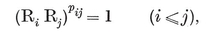
where it is understood that such a relation with pij = ∞ (indicating parallelism of w*i* and w*j*) can be ignored.
If the reflecting hyperplanes fall into two or more sets, such that every two hyperplanes in different sets are perpendicular, then the reflections themselves fall into mutually commutative sets, and the group, being a direct product, is said to be reducible.[image]{.image .placeholder original-image-src=“content/images/00114” original-image-title=“” width=“0in” height=“0in”}irreducible. 120 Thus the irreducible groups in two dimensions are
[1], [p] (p > 2), [ ∞ ], Δ, [4, 4], [3, 6],
and the reducible groups in two dimensions are the direct products
[1] × [1], [∞] × [1], [ ∞ ] × [ ∞ ].
The first step in the general enumeration is to prove that each of the irreducible groups has some kind of simplex for its fundamental region. For this purpose we shall derive a corresponding quadratic form, and use the results of Chapter X.
[image]{.image .placeholder original-image-src=“content/images/00114” original-image-title=“” width=“0in” height=“0in”} The fundamental region is a finite or infinite region bounded by (say) m hyperplanes. Through any point within it, draw lines per-pendicular to all the walls. Let e1, . . . , em be unit vectors along these perpendiculars (directed inwards, from wall to point). Since the angle between ei and ej is the supplement of the dihedral angle π/pij of the fundamental region, we have
ei[image]{.image .placeholder original-image-src=“content/images/00114” original-image-title=“” width=“0in” height=“0in”} ej =–cos π/pij.
[image]{.image .placeholder original-image-src=“content/images/00114” original-image-title=“” width=“0in” height=“0in”}i=j, as well as when i≠j.
If the vectors do not span the whole space, but only a certain subspace, then the reflecting hyperplanes are all perpendicular to this subspace ; so we can take their section by the subspace and consider the same group as operating therein. (For instance, the group generated by reflections in two parallel hyperplanes is essentially the same as that generated by reflections in two points, arising as the section of the hyperplanes by a line perpendicular to both ; thus [ oo ] is to be considered a one-dimensional group.) Having made this remark, we shall assume that the e’s do span the space under consideration, say n-dimensional space. Thus
m ≥ n.
Any m numbers x1, . . . , xm determine with the e’s a vector
x1e1 + . . . + xmemxiei,
whose squared magnitude is
xiei[image]{.image .placeholder original-image-src=“content/images/00114” original-image-title=“” width=“0in” height=“0in”}xkekaik xi xk,
where
[image]
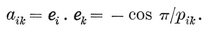
aik xixk can never be negative : it is a positive definite or semidefinite quadratic form in m variables. Since, for i≠k,
–cos π/pik ≤ 0,
this is an a[image]{.image .placeholder original-image-src=“content/images/00114” original-image-title=“” width=“0in” height=“0in”}pik = 2, and therefore aik = 0 ; hence the a-form is connected or disconnected according as the group is irreducible or reducible. We now consider the two possible cases : m=n and m>n.
If m=n, there are only just enough exiei can only vanish when all the x’s vanish; therefore the a-form is positive definite. In this case the n reflecting hyperplanes have a common point, say O. (They cannot contain a common direction instead, as then all the e’s would be perpendicular to that direction, and could not span the space.) We therefore consider the group as acting on a sphere with centre O, and replace its angular fundamental region by an (n–1)-dimensional spherical simplex (e.g., an arc when n=2, as in Fig. 5.1C, and a spherical triangle when n[image]
On the other hand, if m>n, there are too many e’s to be linearly independent, so they must satisfy at least one non-trivial relation
[image]
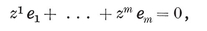
aik zi zk = 0 ; therefore the a-form is positive semidefinite. By a familiar theorem in algebra the n-dimensional vector space is spanned by n of the m e’s ; therefore the a-form has rank n, and nullity m–n. If, further, the group is irreducible, so that the a[image]
m = n + 1.
[image]{.image .placeholder original-image-src=“content/images/00114” original-image-title=“” width=“0in” height=“0in”}z[image]{.image .placeholder original-image-src=“content/images/00114” original-image-title=“” width=“0in” height=“0in”}n-dimensional Euclidean simplex). As we saw in § [image]{.image .placeholder original-image-src=“content/images/00114” original-image-title=“” width=“0in” height=“0in”} the z’s are inversely proportional to the altitudes of the simplex.
We see now that every irreducible group generated by reflections has a simplex for its fundamental region. Since spherical space is finite, whereas Euclidean space is infinite, the group is finite or infinite according as the simplex is spherical or Euclidean. Hence
[image]{.image .placeholder original-image-src=“content/images/00114” original-image-title=“” width=“0in” height=“0in”} Every group generated by reflections is a direct product of groups whose fundamental regions are simplexes. The fundamental region of a finite group generated by reflections is a spherical simplex, and that of an irreducible infinite group generated by reflections is a Euclidean simplex.
[image]
Before enumerating the particular groups, it is worth while to record the following connection between finite and infinite groups. Let G be any infinite discrete group generated by reflections in n-dimensional Euclidean space. The reflecting hyperplanes occur in a finite number of different directions ; for otherwise we could find two of them inclined at an arbitrarily small angle, and the group would not be discrete. In other words, the reflecting hyperplanes belong to a finite number of families, each consisting of parallel hyperplanes. If we represent each family by a single hyperplane (parallel to those of the family) through any fixed point O, we obtain a finite group S, which is generated by reflections in some n of the hyperplanes through O (because its fundamental region is a spherical simplex or n-hedral angle). These represent n particular families of reflecting hyperplanes of G. Instead of hyperplanes through an arbitrary point O, we could have taken one hyperplane from each of these n families. Since there are just n of them, the hyperplanes so chosen meet in a point, and now the fundamental region for S occurs at one corner of the fundamental region for G (which is bounded by these n hyperplanes and one or more others). Thus, however many families of parallel hyperplanes may occur, the fundamental region for G has at least one vertex which lies in one hyperplane of every family. Let us call this a special vertex of the fundamental region, and S a special subgroup of G. Abstractly, S is the largest finite subgroup of G.
To take a simple instance with n = 2, let G be [ ∞ ] × [ ∞ ], generated by reflections in the sides of a rectangle ; then all four vertices of the rectangle are “ special,” and S is [1] × [1], of order 4, generated by reflections in any two adjacent sides. On the other hand, when G is [3, 6] there is only one “ special ” vertex (where the angle π/6 occurs), and S is [6], of order 12.
[image]{.image .placeholder original-image-src=“content/images/00114” original-image-title=“” width=“0in” height=“0in”} We have now reduced the enumeration of discrete groups generated by reflections to that of spherical and Euclidean simplexes whose dihedral angles are submultiples of π[image]{.image .placeholder original-image-src=“content/images/00114” original-image-title=“” width=“0in” height=“0in”}p if p > 3) indicate pairs of walls inclined at angles π/p (p>2). Their perpendicular walls are represented by nodes not joined by a branch. Thus the graph is connected or disconnected according as the group is irreducible or reducible. In the latter case the group is the direct product of several “ irreducible components,” corresponding to the separate pieces of the graph.
The same graph may be regarded as representing the quadratic form. The nodes represent the variables, or the “ square ” terms, and the branches represent the “ product ” terms. (This explains our definition of connected and disconnected[image]
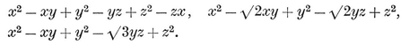
(For simplicity we have written x, y, z instead of x1, x2, x3.)
The graph for a spherical or Euclidean simplex has the property that the removal of any node (along with any branches which emanate from that node) leaves the graph for a spherical simplex. This is geometrically evident, as m–1 of the m[image]{.image .placeholder original-image-src=“content/images/00114” original-image-title=“” width=“0in” height=“0in”}m–1 of the m e’s are linearly independent, even when all the m[image]
[image]{.image .placeholder original-image-src=“content/images/00114” original-image-title=“” width=“0in” height=“0in”} For the application of the above principles we need a standard list of Euclidean simplexes. This list is provided by the right-hand half (W2, etc.) of Table IV on page 297, together with
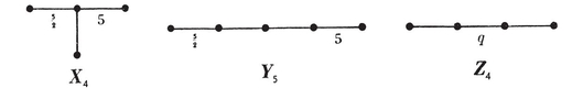
where q is defined by cos π/qPm, Qm, … , Z4 are adapted from Witt 1.) We recognize
P3, P4, R3, R4, S4, V3, W2
as fundamental regions for the respective groups
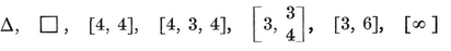
of Chapter V. Most of the rest are natural analogues of these.
All these graphs represent quadratic forms which we shall prove to be semidefinite. It will then follow that they represent Euclidean simplexes. Of course, the three simplexes X4, Y5, Z4 (where fractional marks occur) are not fundamental regions of discrete groups ; nevertheless we shall find them useful.
[image]{.image .placeholder original-image-src=“content/images/00114” original-image-title=“” width=“0in” height=“0in”}aik xi xk is semidefinite if there exist positive numbers z1, … , zm such that
[image]
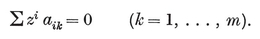
To apply this criterion, we represent the form by its graph, and associate the m z’s with the m nodes.
[image]{.image .placeholder original-image-src=“content/images/00114” original-image-title=“” width=“0in” height=“0in”}kth node is joined by branches to the ith, jth, etc. Then, if these branches are unmarked, so that aik
[image]
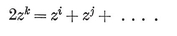
If the “ ikq, we must multiply the zi in the expression by √2, τ, √3, τ–1121[image]{.image .placeholder original-image-src=“content/images/00114” original-image-title=“” width=“0in” height=“0in”}z’s are in arithmetical progression.
After these instructions, it takes only a few minutes to insert the appropriate z’s at the nodes of the graphs in the table on page 194, which shows that Pm, Qm, . . . , Z4 are in fact Euclidean simplexes (in space of m–1 dimensions).
[image]{.image .placeholder original-image-src=“content/images/00114” original-image-title=“” width=“0in” height=“0in”}z’s, we are at liberty to “ normalize ” these m[image]{.image .placeholder original-image-src=“content/images/00114” original-image-title=“” width=“0in” height=“0in”}zi = 1 and all the z’s are uniquely determined.
[image]{.image .placeholder original-image-src=“content/images/00114” original-image-title=“” width=“0in” height=“0in”} From these Euclidean simplexes we can derive spherical simplexes by drawing spheres round the vertices, i.e., by removing a node from each graph. Since it will suffice to enumerate irreducible groups, we only remove such nodes as will leave the graph connected. By removing one of the nodes marked 1 from each graph in the table on page 194, we find that the Euclidean simplexes
W2, Pn+1, Qn+1,T7, T8,T9,Rn+1 or Sn+1, U5, V3, X4, Y5,
yield the spherical simplexes

of Table IV.
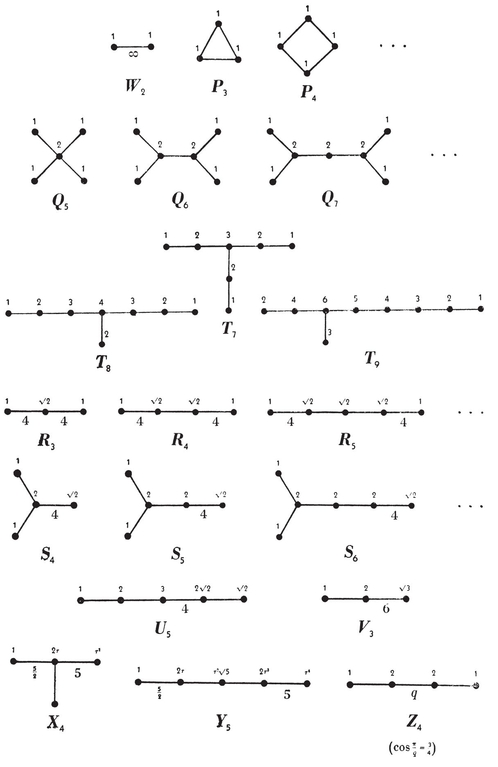
We recognise A1, A2, A3, C2, C3G3[image]{.image .placeholder original-image-src=“content/images/00114” original-image-title=“” width=“0in” height=“0in”}π/p) which are fundamental regions for the “ non-crystallographic ” dihedral groups [p] (p=5, 7, 8, … ).
To make sure that the enumeration of irreducible groups is now complete, we consider the possibility of a further graph, and employ the principle that such a graph cannot be derivable from the graph for a Euclidean simplex by adding new branches, nor by increasing the marks on old branches. Since Pm is Euclidean, the new graph must be a tree[image]{.image .placeholder original-image-src=“content/images/00114” original-image-title=“” width=“0in” height=“0in”}A1, W2A2C2) have already been mentioned, the tree must have at least two branches. Since Qm is Euclidean, there cannot be as many as four branches at any node, nor as many as three at each of two nodes. If there is one node where three branches meet, the tree consists of three chains radiating from that node, say i branches in one chain, j in another, k in the third, with i ≤ j ≤ k. Since Sm is Euclidean, none of these branches can be marked. Since Bn has already been mentioned, j > 1 ; since T7 is Euclidean, i = 1 ; since T8 is Euclidean, j = 2 ; and since T9 is Euclidean, k < 5. But E6, E7, E8 have already been mentioned, so the possibility of three branches at a node is ruled out.
We now have to consider a single chain. Since An has already been mentioned, and Rm is Euclidean, there must be just one marked branch. Since V3 and U5, are Euclidean, the mark can only be 4 or 5, and must occur on an “ end ” branch or on the middle one of three. Since Cn and F4 have already been mentioned, the mark can only be 5. Since Y5G3 and G4 have already been mentioned, so we are forced to return to the case of a chain of three branches with the middle one marked. Since Z4 is Euclidean (and q<5), this last possibility is ruled out. To sum up our important result :
The only irreducible discrete groups generated by reflections are those whose fundamental regions are the spherical simplexes
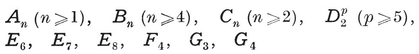
(see Table IV on page 297) and the Euclidean simplexes
W2, Pm (m ≥3), Qm (m ≥ 5), Rm (m ≥ 3), Sm (m ≥ 4),
V3, T7, T8, T9, U5.
In the following paragraphs we shall relate each of the finite groups to a polytope, and thence compute its order.
[image]{.image .placeholder original-image-src=“content/images/00114” original-image-title=“” width=“0in” height=“0in”}[image]
In the case of an (m–1)-dimensional spherical simplex, the polytope need not be properly m-dimensional. If it is n-dimensional, where n<m, the group leaves invariant an n-dimensional subspace of the m-dimensional Euclidean space ; then every reflecting hyperplane either contains this subspace or is perpendicular to it, so the group is reducible. Conversely, if the group is reducible, so that the graph is disconnected, suppose that the piece containing the ringed node has altogether n nodes. Then the group has an irreducible component generated by the corresponding n reflections, and this yields the n-dimensional polytope represented by the ringed piece. The rest of the graph may be disregarded ; for, the corresponding m–n hyperplanes each contain the whole polytope, so the reflections in them have no effect on it.
In the case of an (m–1)-dimensional Euclidean simplex, the honeycomb is necessarily (m–1)-dimensional. For if the group were reducible its fundamental region would not be a simplex.
In order to treat polytopes and honeycombs simultaneously, we restrict consideration to irreducible groups, and regard the polytopes as having been projected radially onto their circum-spheres ; i.e., we consider (m–1)-dimensional spherical and Euclidean honeycombs. In either case, the symbol consists of a connected graph having m nodes, of which one is ringed.
A typical edge (of the honeycomb) joins the chosen vertex to its image by reflection in the opposite wall of the fundamental region. Thus every edge is perpendicularly bisected by one of the reflecting hyperplanes, i.e., by an actual or virtual mirror of the generalized kaleidoscope. This holds, in particular, for all the edges of any cell, Π*m*–1; but in their case all the hyperplanes pass through the centre, P, of that cell. We thus have at least m–1 linearly independent reflecting hyperplanes through P (e.g., those bisecting the edges of Π*m*–1 that meet at one vertex). Hence P may be taken to be a vertex of the fundamental region, and the symbol for the cell is derived from the symbol for the whole honeycomb (or polytope) by removing the node that represents this vertex (and of course removing also every branch which occurs at that node).
Conversely, the removal of an unringed node from the symbol for a polytope or honeycomb leaves the symbol for an element Π*k*, which is a cell (k = m–1) if the graph remains connected. The only case (with m > 2) in which every unringed node yields a cell, is when the original graph is an m-gon (so that the fundamental region is the Pm of Table IV) ; in every other case the graph is a tree, and there is a cell for each free end, i.e., for each unringed node that belongs to only one branch. Similarly, the removal of a free end from the symbol for a Π*m*–1 leaves the symbol for a Π*m*–2, and so on. Finally, the ringed node by itself represents an edge, Π**1, and its removal leaves the null graph (i.e., nothing at all), which represents a vertex, Π0**.
Thus every type of element Π*k* is derivable by removing a certain number of nodes from the symbol for the whole polytope or honeycomb. So far as the element itself is concerned, any unringed piece of the graph may be disregarded. But when we come to compute the number of elements of that type, the unringed pieces become important, and must be fully restored (for a reason that will appear soon). According to this rule, the maximum number of nodes that may be removed simultaneously is equal to the number of free ends, except in the case of Pm k, while the nodes of any unringed pieces represent hyperplanes which contain the Π*k. Thus the graph for the Πk, regardless of the ring, represents the fundamental region for the subgroup leaving the Πk* invariant. The various equivalent Π*k’s correspond to the cosets of this subgroup. Hence the number of such Πk*[image]
In particular, the symbol for a vertex is derived by removing the ringed node. The resulting unringed graph could just as well be the null graph so far as the kind of element is concerned ; but the corresponding group is the subgroup that leaves the vertex invariant (for it is generated by reflections in hyperplanes through the vertex). The number of vertices is equal to the index of this subgroup.
When the ringed node belongs to only one branch, we can go a step further, and obtain a symbol for the vertex figure[image]{.image .placeholder original-image-src=“content/images/00114” original-image-title=“” width=“0in” height=“0in”}first node, and suppose the only branch from it goes to the second. These two nodes represent vertices P0 and P1 of the fundamental region, namely a vertex of the honeycomb (or polytope) and the mid-point of an edge. The vertices of the vertex figure are the mid-points of all the edges that meet at P0, i.e., the transforms of P1 by the subgroup that leaves P0 invariant. Hence we obtain the vertex figure by removing the first node (along with its branch) and transferring the ring to the second node.
[image]{.image .placeholder original-image-src=“content/images/00114” original-image-title=“” width=“0in” height=“0in”} We can now prove that the polytope or honeycomb
[image]
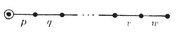
is regular, being in fact the same as {p, q, . . . , v, w[image]{.image .placeholder original-image-src=“content/images/00114” original-image-title=“” width=“0in” height=“0in”}p-gon {p p, q[image]

Each kind of element can be obtained by removing a single node, in fact the k-dimensional element is given by removing the (k + 1)th node. We thus see again, more clearly than on page 140, that the orthoscheme
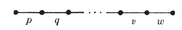
is the characteristic simplex of the regular polytope
{p, q, . . . , v, w},
whose symmetry group
[p, q, … , v, w]
is generated by reflections in the bounding hyperplanes of that orthoscheme.122
[image]
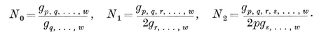
[image]{.image .placeholder original-image-src=“content/images/00114” original-image-title=“” width=“0in” height=“0in”}Δp, *q*, . . . , *w* is the determinant of the a-form
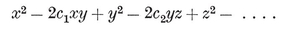
[image]
The polytope
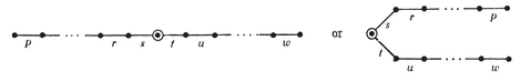
whose vertices are the centres of the {p, … , r}’s of {p, … , w[image]

which is the regular polytope {w, . . . , p}, reciprocal to {p, . . . , w}.
We have seen that the finite groups

have fundamental regions An, CnF4, G3, G4 (defined in Table IV, page 297). By a convenient extension of this notation we shall use the symbols
[3k, 1, 1] [32 , 2, 1], [33, 2, 1], [34, 2, 1]
for the groups whose fundamental regions are Bk+3, E6, E7, E8.
In Fig. 5.4A we split an isosceles spherical triangle into two equal parts, symbolically
[image]

and deduced that [3, 3] is a subgroup of index 2 in [3, 4]. Analogously, the spherical tetrahedron B4 is symmetrical by reflection in the bisector of one of its dihedral angles, and is thereby split into two C4’s. More generally
[image]

and therefore [3*n*–3, 1, 1] is a subgroup of index 2 in [3*n*–2, 4]. Thus the order of [3*n*–3, 1, 1] is
[image]

(Since B3 is the same as A3[image]
There is a similar relation between pairs of infinite groups, since
P3 =2V3, Qn = 2Sn, and Sn = 2Rn.
(We saw in Fig. 4.7A that P4 = 2S4. The symbol Q4 has not been defined, so we are free to identify it with P4. The shape of the graph makes this quite reasonable.)
It follows that the polytope and honeycombs
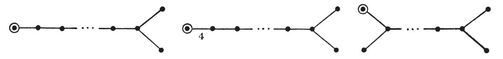
are the same as
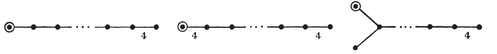
while the vertices of the third of them are alternate vertices of the second. In fact, these are β*n, δn, hδn*[image]
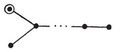
is hγ*n*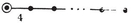 γn.
γn.
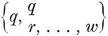
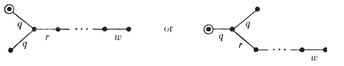

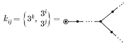
which implies
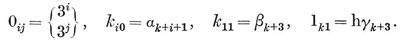
By removing two nodes from the graph, we find that the number of 0*ab’s in 0ij* is equal to the coefficient of Xi−a Yj−b in (1+X+Y)*i*+*j*+2 ; e.g., the number of edges 000 is the coefficient of X*i* Y*j.* But the number of vertices is the coefficient of Xi+1 Yj+1.[image]{.image .placeholder original-image-src=“content/images/00114” original-image-title=“” width=“0in” height=“0in”}kij is (k−1)ij. To include the case where k=0, we may write (−1)ij=a*i×aj*.
[image]{.image .placeholder original-image-src=“content/images/00114” original-image-title=“” width=“0in” height=“0in”} The simplest polytopes arising from the finite groups [32, 2, 1], [33, 2, 1], [34, 2, 1] are 221, 321, 421 ; and the simplest honeycombs arising from the infinite groups [32, 2, 2], [33, 3, 1], [35, 2, 1] are 222, 331, 521. These polytopes and honeycombs (in six, seven, and eight dimensions)123 are not related to any regular figures (of the same number of dimensions) ; but we shall consider them briefly as a means to compute the orders, say x, y, z, of the groups [32, 2, 1], [33, 2, 1], [34, 2, 1].
The six-dimensional polytope 221 has cells of two kinds, both regular :
220=α5, 211=β5.
The number of elements of any kind may be expressed in terms of the unknown order x by removing one or two nodes from the graph
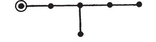
as in the following table :
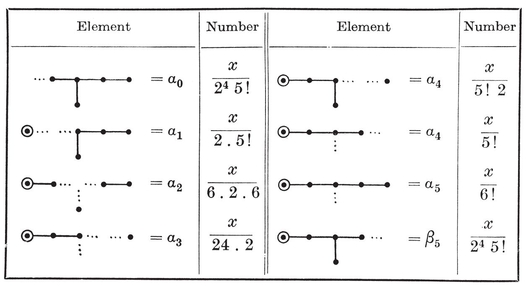
Thus
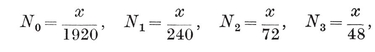
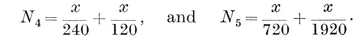
“ Euler’s Formula ” N0 − N1 + N2 − N3 + N4 − N5[image]{.image .placeholder original-image-src=“content/images/00114” original-image-title=“” width=“0in” height=“0in”}n = 6) is satisfied identically, and so does not help us to compute x.
Not discouraged by this initial setback, we make a similar table for the honeycomb 222, and obtain the proportional numbers of elements
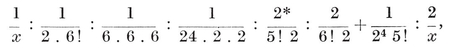
or, after multiplication by 24 . 6 ! ,

[image]
whence
ν0 − ν1 + ν2 − ν3 + ν4 − ν5 + ν6 = 0,
[image]
Thus 221 has 27 vertices, 216 edges, 720 triangles, 1080 tetrahedra, 216+432 α4’s, 72 α5’s and 27 (β5’S. (See Coxeter 14.)
Similarly, the seven-dimensional polytope 321 has
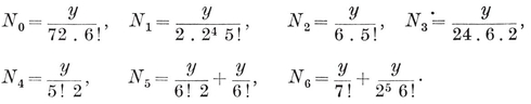
(The cells are 320=α6 and 311=β6.) The equation
N0 − N1 + N2 − N3 + N4 − N5 + N6 = 2
yields
[image]

Thus 321 has 56 vertices, 756 edges, … , 2016+4032 α5’s, 576 α6’s and 126 β6’s. (See Coxeter 1, p. 7.)
Again, the eight-dimensional polytope 421 has
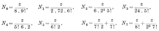
(with cells 420=α7 and 411=β7). Euler’s Formula is satisfied, regardless of the value of z. But the honeycomb 521 has the proportional numbers
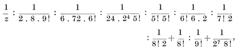
or, after multiplication by 192 . 10 ! ,
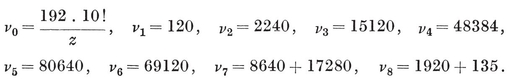
From the equation ν0 − ν1 + ν2 − ν3 + ν4 − ν5 + ν6 − ν7 + ν8 = 0 we deduce
[image]
Thus 421 has 240 vertices, 6720 edges, … , 69120+138240 α6’s, 17280 α7’s and 2160 β7’s. (See Gosset 1, p. 48.)
This completes our computation of the orders of the finite groups generated by reflections, as given in Table IV (page 297).
1[image]{.image .placeholder original-image-src=“content/images/00114” original-image-title=“” width=“0in” height=“0in”} The above method for computing the order of [3*k*, 2, 1[image]{.image .placeholder original-image-src=“content/images/00114” original-image-title=“” width=“0in” height=“0in”}π/2 or π/3, and the graph has no marked branches. We shall find that the order of the special subgroup of a trigonal group in n dimensions is
[image]
where f[image]{.image .placeholder original-image-src=“content/images/00114” original-image-title=“” width=“0in” height=“0in”}f special nodes, and we shall see that these are just the nodes for which zi[image]
Let S be the special subgroup of an irreducible infinite group G,[image]{.image .placeholder original-image-src=“content/images/00114” original-image-title=“” width=“0in” height=“0in”}G is a simplex, and the corresponding graph is connected). Then S consists of those operations of G which preserve a special vertex 0 of the fundamental region, and this subgroup S is isomorphic to the quotient group G/T, where T consists of all the translations in G. (Cf. Burckhardt 2, p. 103.)
The fundamental region for G, being a simplex, is bounded by n+1 hyperplanes, n of which pass through 0. Reflections in these n generate S, while the remaining one serves to reflect 0 into another “ special ” point O′. Thus 00′ is an edge of the honeycomb125 whose symbol is derived from the graph by ringing the O-node, and this edge is perpendicularly bisected by one of the reflecting hyperplanes of G. The reflection in the parallel hyperplane through 0 must likewise belong to G (in fact, to S). The product of these two reflections is the translation from 0’ to O. Since any vertex of the honeycomb can be reached by a path along a sequence of edges, the subgroup T is generated by translations along edges. Thus the vertices, which are the transforms of 0 by G, are also the transforms of 0 by T ; this shows that they form a lattice.
A typical cell of the reciprocal honeycomb is a polytope having 0 for in-centre. Its bounding hyperplanes perpendicularly bisect the lines joining O to the nearest other lattice points (which are the transforms of O′ by S). Its simplicial subdivision consists of repetitions of the fundamental region for G, in number equal to the order of S. The polytope, being a fundamental region for T, has the same n-dimensional content as a “ period parallelotope ”. The order of S is the ratio of this content to that of the fundamental region for G (in agreement with the fact that this order is equal to the index of T in G).
We have seen that the reflecting hyperplanes of G occur in various families of parallel hyperplanes. Suppose the fundamental region has f special vertices. If f=1 the points of the above lattice are the only points which lie in representative hyperplanes of every family. But in general the totality of such special points consists of f superposed lattices, which together form a single lattice of finer mesh.
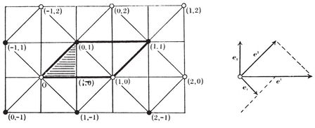
This is still a lattice. For, the reflecting hyperplanes through any two special points are respectively parallel ; so there must be a translation carrying the one special point to the other, even if this translation does not occur in T. (In fact, the translation transforms G according to an automorphism, which need not be an inner automorphism.)
The situation is illustrated in Fig. 11.9A, where G is [4, 4], so that S is [4], of order 8. Here the fundamental region is a right-angled isosceles triangle, and *f=*2. The two special vertices are transformed into the “ white ” and “ black ” points, respectively. These form two lattices, which are the vertices of two reciprocal {4, 4}’s. The “ polytope having 0 for in-centre ” is a face of the black {4, 4}, and at the same time serves as a period parallelogram for T. Its area is plainly 8 times that of the right-angled isosceles triangle. The “ lattice of finer mesh ” consists of the white and black points together, forming a smaller {4, 4}.
Since f lattices (of transforms of O by T or G) are superposed to make the lattice of all special points, the period parallelotope of the former is f times as large as that of the latter. The smaller period parallelotope is bounded by the hyperplanes of the n generating reflections of S and by n further hyperplanes parallel. to these (the next in the respective families). We now choose a system of affine coordinates in such a way that these 2n hyperplanes are
x*i* =0 and x*i* = 1 (i = 1, 2, . . . , n).
Then the special points are just the points whose covariant coordinates are integers (as in Fig. 11.9A). The contravariant vectors e*i*, which determine these coordinates, proceed along the edges through 0 of the fundamental region, and are of such magnitudes as to reach the nearest special points along those edges.126
The fundamental region for G is bounded by the n hyperplanes, x*i* = 0 and by one further hyperplane, say
[image]
The edges through O represent vectors
e1/y1, . . . , en/y*n*,
which lead to the vertices (1/y1, 0, . . . , 0, 0), … , (0, 0, … , 1/yn). The content of the simplex is 1/n! times that of the parallelotope based on these vectors. This, in turn, is 1*/*(y1 … yn) times the content of the parallelotope based on e1, … , en, which is 1/f times that of the fundamental region for T. Hence the order of S is
[image]
where yi is the number of times the ith edge through O (of the fundamental region for G) has to be produced before we come to another special point. In particular, yi=1 if the edge joins O to a second special vertex, but otherwise y*i* > 1.
The hyperplane through O[image]{.image .placeholder original-image-src=“content/images/00114” original-image-title=“” width=“0in” height=“0in”}yi xi = 0. Hence the family of hyperplanes to which these belong is given by
yi xi = j,
where jyi xi must be an integer for all integral values of the x’s. Hence the y’s are integers.
Can these n positive integers be determined without a detailed examination of the reflecting hyperplanes ? Is there some algebraic rule for deriving them straight from the graph ? Such a rule has not been found in the general case, but only when G is a trigonal group (so that the graph has no marked branches). In this case we use unit vectors e1, . . . , e*n*+1, perpendicular to the bounding hyperplanes of the fundamental region O1 . . . On+1[image]{.image .placeholder original-image-src=“content/images/00114” original-image-title=“” width=“0in” height=“0in”}O*n*+1 is a special vertex. We may also take the altitude from this vertex as our unit of length, so that
[image]

Then the bounding hyperplane xn+1 = 0 or
[image]
is one of the reflecting hyperplanes of G, and the parallel hyperplane through O*n*+1 is x*n*+1 = 1 or z1 x1 + … + Zn xn[image]{.image .placeholder original-image-src=“content/images/00114” original-image-title=“” width=“0in” height=“0in”}x1, . . . , xn are integers.
[image]{.image .placeholder original-image-src=“content/images/00114” original-image-title=“” width=“0in” height=“0in”}O1 . . . O*n*+1[image]
[image]
where m=n[image]{.image .placeholder original-image-src=“content/images/00114” original-image-title=“” width=“0in” height=“0in”}127 yi = zi[image]
We now understand why it always happens that the z’s (for the trigonal groups) are integers. (See the table on page 194.) Moreover, the special nodes are those for which zi = 1. Re-moving one of these in each particular case, we verify that the finite groups
[3n−1], [3n−3, 1, 1], [32, 2, 1], [33, 2, 1], [34, 2, 1],
whose fundamental regions are
An, Bn, E6, E7, E8,
are the special subgroups of the infinite groups whose fundamental regions are
Pn+1, Qn+1, T7, T8, T9.
[image]
¶ –
Thus the computation of the orders of the trigonal groups no longer presents any difficulty. On the other hand, a glance at Table IV shows that all the finite non-trigonal groups are symmetry groups of regular polytopes. These have already been studied separately in Chapter VIII. The four-dimensional groups [p, q, r],[image]
[image]{.image .placeholder original-image-src=“content/images/00114” original-image-title=“” width=“0in” height=“0in”} The finite groups generated by reflections in four-dimensional Euclidean space (or in three-dimensional spherical space) were first enumerated in 1889, by Goursat,129 whose knowledge of the regular polytopes was derived from Stringham 1. The analogous groups in n dimensions were considered in 1928 by Cartan (2), who showed that the fundamental region must be a simplex. The completeness of his enumeration was verified in a direct geometrical manner three years later (Coxeter 2),[image]{.image .placeholder original-image-src=“content/images/00114” original-image-title=“” width=“0in” height=“0in”}aik).
[image]{.image .placeholder original-image-src=“content/images/00114” original-image-title=“” width=“0in” height=“0in”}k corresponds to the insertion of a ring, and her “ contraction ” c to the removal of a ring. The reason for this was lucidly explained by G. de B. Robinson (1, p. 72). Wythoff himself was largely concerned with the group [3, 3, 5], but he added the remark that “ a similar investigation … may be undertaken in the same manner with regard to the other polytope-families in four-dimensional and in other spaces ”. (Wythoff 2, p. 970.)
Gosset’s polytopes k21[image]{.image .placeholder original-image-src=“content/images/00114” original-image-title=“” width=“0in” height=“0in”}130 in 1911, along with the remaining polytopes kij (except 142, which fails to satisfy Elte’s rather artificial definition of “ semi-regular ”). Their symmetry groups [3*k,* 2, 1] were investigated at about the same time by Burnside, qua groups of rational linear transformations of n variables (n=k+4). His tables (Burnside 2, pp. 301, 304, 307) may be interpreted as an enumeration of the 72 α5’s of 221, the 576 α6’s of 321, and the 17280 α7’s of 421 ; but he did not give them this interpretation himself. If he had finished reading Gosset’s essay (see page 164), he would surely have seen the connection. Moreover, he and Baker described two dual configurations131
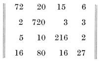
and
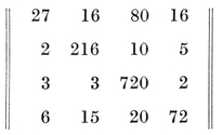
in projective four-space, which show a remarkable resemblance to 122 and 221. In 1932, Room (1, p. 152) considered two five-dimensional configurations which are still more closely related to these polytopes (though he was not aware of this). J. A. Todd (2) made use of Room’s configurations in his proof that [32, 2, 1] is isomorphic with the group of incidence-preserving permutations of the 27 lines on the general cubic surface. (For the earliest description of these lines, see Schläfli 2.) Todd thus explained the fact, noticed by Schoute (9) in 1910, that the tactical relations between the 27 lines can be exhibited as relations between the 27 vertices of Gosset’s six-dimensional polytope 221. Du Val (1, p. 69) generalized this result, relating the vertices of (5−m)21 to the lines on the del Pezzo surface of order m in projective m-space. He showed also that the 28 pairs of opposite vertices of 321 correspond to the 28 bitangents of the general plane quartic curve (cf. Coxeter 1), while the 120 pairs of opposite vertices of 421 (or the 120 reflections of [34, 2, 1]) correspond to the 120 tritangent planes of the twisted sextic curve in which a cubic surface meets a quadric cone.
The vertices of Gosset’s eight-dimensional honeycomb 521 (of edge √2) have as coordinates all sets of eight integers or eight halves of odd integers, with an even sum. (See Coxeter 1, p. 2, where 521 is called (PA)9.) This lattice not only has the same shape[image]{.image .placeholder original-image-src=“content/images/00114” original-image-title=“” width=“0in” height=“0in”}coincides with its reciprocal (like the cubic lattice of edge 1). The same points, in a different coordinate system, represent the integral Cayley numbers (Coxeter 16) in the same way that the vertices of {4, 4} and {3, 3, 4, 3} represent the Gaussian integers and integral quaternions.
Weyl (1) represented the operations of a semi-simple continuous group (or Lie group) by the points of a certain manifold. Cartan (1, pp. 215-230) deduced that for each semi-simple Lie group there is a corresponding infinite group generated by reflections, with a finite fundamental region. Our direct enumeration of such groups shows that he used them all. In fact, there is a one-to-one correspondence between (i) families of locally isomorphic simple [or semi-simple] Lie groups with complex parameters and (ii) reflection groups whose fundamental regions are simplexes [or rectangular products of simplexes] in Euclidean space. (See Stiefel 1.) In particular, the “ classical ” groups (Weyl 2) corresponds to simplexes as follows :
¶ –
[image]{.image .placeholder original-image-src=“content/images/00114” original-image-title=“” width=“0in” height=“0in”}G, S, T. His § is the fundamental region for G.O. It should be emphasized that his coordinates for 222 (“ type E6 ”, p. 230) are oblique, although those for 331 and 521 are rectangular. His h (the “ connectivity ” of the group manifold) is our f = det(2aik). His m1, . . . , ml (Cartan 2, p. 256) are the y1, . . . , yn[image]
These y‘[image]{.image .placeholder original-image-src=“content/images/00114” original-image-title=“” width=“0in” height=“0in”}product. Here is another, involving their sum : the total number of families of parallel hyperplanes in an infinite group G (or the total number of reflections in the special subgroup S) is

e.g., the number of families in [35, 2, 1], or of reflections in [34, 2, 1 2). It is equivalent to the statement that the number of parameters (Gliederzahl) of a simple continuous group is
(2 + y1+ y2+ . . . +yn)n.
We have already seen that, in the important case of the trigonal groups, these y[image]{.image .placeholder original-image-src=“content/images/00114” original-image-title=“” width=“0in” height=“0in”}Table IV) also represent the neighbourhoods of an important kind of singular point on an algebraic surface. The numbers zi occur as the coefficients of the partial neighbourhoods in the expression for the whole neighbourhood.
[]
¶ CHAPTER XII
THE GENERALIZED PETRIE POLYGON
[image]{.image .placeholder original-image-src=“content/images/00114” original-image-title=“” width=“0in” height=“0in”}p, q, r[image]{.image .placeholder original-image-src=“content/images/00114” original-image-title=“” width=“0in” height=“0in”}p, q, r}.[image]
[image]{.image .placeholder original-image-src=“content/images/00114” original-image-title=“” width=“0in” height=“0in”} In n dimensions, as in three, a congruent transformation is a point-to-point correspondence preserving distance. It consequently preserves collinearity, i.e., it is a special kind of collineation. It is determined by its effect on an n-dimensional n[image]{.image .placeholder original-image-src=“content/images/00114” original-image-title=“” width=“0in” height=“0in”}n+ 1 reflections. Again it is direct or opposite (i.e., a displacement or an enantiomorphous transformation) according as the number of reflections is even or odd.
The special case when there is at least one invariant point is called an orthogonal transformation. This is the product of at most n reflections (in hyperplanes through the invariant point). In terms cf affine coordinates with their origin at the invariant point, it is a linear transformation
[image]
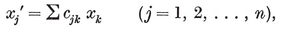
where the coefficients Cjk[image]
[image]{.image .placeholder original-image-src=“content/images/00114” original-image-title=“” width=“0in” height=“0in”}n equations
[image]
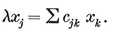
The first step in solving these is to eliminate the x’s, obtaining a single equation of the nth degree in λ :
[image]
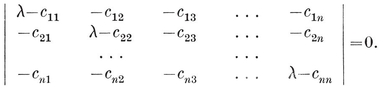
Each root of this equation yields a value of λ which we can substitute in the n equations [image]{.image .placeholder original-image-src=“content/images/00114” original-image-title=“” width=“0in” height=“0in”} (at least one of which will be redundant) ; then we can solve for the x’s and so obtain an invariant direction.
A real root gives a real vector, and an imaginary root an imaginary vector. In order to take the latter into consideration, we suppose our real Euclidean n-space to be embedded in a complex Euclidean n-space.
[image]{.image .placeholder original-image-src=“content/images/00114” original-image-title=“” width=“0in” height=“0in”}characteristic roots, the corresponding vectors are called characteristic vectors,[image]{.image .placeholder original-image-src=“content/images/00114” original-image-title=“” width=“0in” height=“0in”}characteristic equation. The transformation preserves (or reverses) the direction of each characteristic vector, but multiplies its magnitude by a definite number, which is the characteristic root. Being geometrical properties of the transformation, the characteristic roots are invariants, independent of the chosen coordinate system ; in particular, they are the same whether the coordinates be rectangular or oblique.
Any linear transformation has characteristic roots. One special feature of an orthogonal transformation is that its characteristic roots have unit modulus : λ = 1. This can be seen as follows.
If [image]{.image .placeholder original-image-src=“content/images/00114” original-image-title=“” width=“0in” height=“0in”} is an orthogonal transformation, it preserves the inner product of any two vectors. (Since the characteristic roots are invariants, we are at liberty to use rectangular Cartesian coordinates.) If two vectors x and y are transformed into x′ and y’, the inner products are
x · yxk ykkl xk yl
and
x′ · y′j′ y*j′cjk* xkjl ylcjk cjl xk y*l.*
The conditions for these to be equal are
[image]

[image]{.image .placeholder original-image-src=“content/images/00114” original-image-title=“” width=“0in” height=“0in”}xj by its complex conjugate
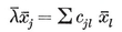
and summing, we have

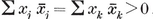
[image]
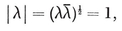
as we wished to prove.
[image]{.image .placeholder original-image-src=“content/images/00114” original-image-title=“” width=“0in” height=“0in”}orthogonal transformation. An important instance is the rotation (through angle ξ)
[image]
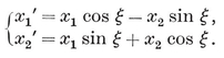
Here the characteristic equation is (λ−cos ξ)2+sin2 ξ=0, and its roots are
cos ξ ± i sin ξ = e±*ξi*.
We proceed to show how any orthogonal transformation can be expressed as a product of commutative rotations and reflections. This is closely related to the algebraic theorem that every polynomial with real coefficients can be expressed as a product of real quadratic and linear factors.
For an imaginary characteristic root we can find at least one characteristic vector. (If there are many, choose one at random.) Its complex conjugate vector has likewise an invariant direction, and the two together span a real invariant plane (through the origin). Let us choose two real perpendicular vectors in this plane as axes of x1 and x2, and insist that the remaining n−2 axes shall lie in the completely orthogonal (n−[image]
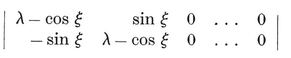
After removing the factor (λ−cos ξ)2 + sin2 ξ = (λ− eiξ)(λ− e−iξ), we are left with the characteristic equation of the transformation induced in the completely orthogonal (*n–*2)-space. If this (n–2)-ic equation still has an imaginary root, we repeat the process, choosing axes of x3 and x4 in a second invariant plane. Proceeding thus we see that, if there are q pairs of conjugate imaginary roots e±*iξk* (k = 1, . . . , q), and n—2q real roots ± 1, then we can analyse the orthogonal transformation into rotations through angles ξk in the planes of the axes of x2*k*−1 and x2*k*, along with a specially simple kind of orthogonal transformation in the residual (n − 2q)-space
x1 = . . . = x2*q* = 0,
where the characteristic roots are only ± 1.
Any real characteristic root provides a real characteristic vector which is preserved or reversed by the orthogonal transformation. We use this to define one of the remaining axes, and then turn our attention similarly to the perpendicular (n−2q−1)-space. We thus obtain orthogonal axes of x2*q*+1, . . . , xn, each of which is either preserved or reversed :
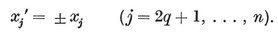
The signs of the various xj’s agree with the signs of the corresponding characteristic roots. Hence, if the n−2q real roots consist of r (−1)’s and n−2q−r 1’s, so that the characteristic equation is
(λ2− 2λ cos ξ1 + 1) . . . (λ2 − 2A cos ξq + 1)(A + 1)r (λ − 1)*n*−2*q*−*r* = 0 ,
then the transformation consists of q rotations and r reflections, all commutative with one another.
Since a rotation preserves sense, while a reflection reverses sense, the above orthogonal transformation is direct or opposite according as r is even or odd. In particular, the general displacement preserving the origin in four dimensions is a double rotation,132 expressible in the form
x1′= x1 cos ξ1 − x2 sin ξ1, x3′ = x3 cos ξ2 − x4 sin ξ2,
x2′ = x1 sin ξ1 + x2 cos ξ1, x4′ = x3 sin ξ2 + x4 cos ξ2.
The two completely orthogonal planes of rotation are uniquely determined except when ξ2= ±ξ1, in which case only two (instead of three) of the four equations 12·12 are independent, and we have a Clifford displacement (analogous to the “ Clifford translation ” of elliptic geometry) The cases when two or four characteristic roots are real are covered by allowing ξ1 or ξ2 to take the extreme values 0 and π.
12·2. Congruent transformations. As a temporary notation, let Q denote a rotation, R a reflection, T a translation, and let Q*q* R*r* T denote a product of several such transformations, all commutative with one another. Then RT is a glide-reflection (in two or three dimensions), QR is a rotatory-reflection, QT is a screw-displacement, and Q2 is a double rotation (in four dimensions). Having proved that every orthogonal transformation is expressible as
Q*q* R*r* (2q + r ≤ n),
we shall not find much difficulty in deducing that every congruent transformation is either
Q*q* R*r* (2q + r ≤ n) or Q*q* R*r* T (2q + r + 1 ≤ n).
The complete statement is as follows :
12·21. In an even number of dimensions every displacement is either Qq Rr (2q + r ≤ n*,* r even*)* or Qq Rr T (2q + r ≤ n − 2, r even*)* and every enantiomorphous transformation is Qq Rr T (2q + r ≤ n − 1, r odd*).* In an odd number of dimensions every enantiomorphous transformation is either Qq Rr (2q + r ≤ n*,* r odd*)* or Qq Rr T (2q + r ≤ n − 2, r odd*)* and every displacement is Qq Rr T (2q + r ≤ n − 1, r even*).*
(We admit Q*q* R*r* as a special case of Q*q* R*r* T by allowing the extent of the translation to vanish.)
In § 3·1 we proved this for the cases n=2 and n=3. So now we use induction, assuming the result in the next lower number of dimensions. For brevity, we consider two cases simultaneously, writing alternative words in square brackets.
If n is even [odd], the general direct [opposite] transformation, being the product of at most n reflections, leaves invariant either a point or two parallel hyperplanes (i.e., either an ordinary point or a point at infinity). In the former case we have the orthogonal transformation Q*q* R*r, where 2q*+r ≤ n. In the latter the transformation is essentially (n−1)-dimensional ; by the inductive assumption it is Q*q* R*r* T, where 2q+r ≤ n−2.
Again, n being even [odd], the general opposite [direct] transformation may at first be regarded as operating on bundles of parallel rays, represented by single rays through a fixed point O. The induced orthogonal transformation is Q*q* R*r, where 2q*+r ≤ n ; but r is odd [even], so 2q+r ≤ n−1. Hence the induced transformation has an invariant axis (“ the nq R*r* or Q*q* R*rq* R*r*−1 T or Q*q* R*r*−1 T2, where T2 means the product of two translations, both commutative with all the Q’s and R’s, so that T2 can be written simply as T.
This completes the proof of 12·21. Since the product of two commutative reflections is a rotation through angle π, while the identity is a rotation through angle 0, an alternative enunciation (like 3·13 and 3·14) can be made as follows.
In 2q dimensions every displacement is Qq or Qq−*1* T, and every enantiomorphous transformation is Qq−*1* RT. In 2q*+1* dimensions every displacement is Qq T, and every enantiomorphous transformation is Qq R or Qq−*1* RT.
12·3. The product of n reflections. A particular orthogonal transformation which is relevant to the study of regular polytopes (for a reason that will appear in § 12·4) is the product R1 R2 . . . R*n* of the generators of a finite group generated by reflections. This, being the product of nn is even or odd. (Here the Q’s stand for commutative rotations, through angles ξk which remain to be computed.) In terms of coordinates x1, x2, . . . , xn, which are distances from the reflecting hyperplanes, the reflection R*k* is given by 10·63 or
xj = x*j′* − 2ajk xk′ ,
where − ajk is the cosine of the dihedral angle between the jth and kth hyperplanes (and akk = 1). Thus R1 R2 . . . R*n* transforms
(x1, x2, . . . , xn) into (x1(*n*), x2(*n*), . . . xn(*n*)),
where xj(*n*) is given indirectly by the n sets of equations
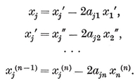
The general case is treated elsewhere.133 For simplicity, let us here restrict consideration to the case when the group is [p, q, … , w], so that the only non-vanishing ajk’s with j < k are

Then the above n2 equations become
12·31
whence, for any value of λ,
12·32
Now, the characteristic equation 12·13 is the result of eliminating he xjxj = xj′ and 12·11. Hence the characteristic equation for R1 R2 … R*n* can be obtained by eliminating all the xj(*k*)’s from
λxj = xj*(*n*)*
and 12·31. By means of 12·32, all the xj(k)’s for which j≠k are eliminated automatically, and we are left with the n equations
or

In the extreme cases where j=1 or n, the first or last term will be lacking. Eliminating the y’s from
we obtain the characteristic equation
12·33
or, in the notation of 7·76,
12·34
Here X ξk of the component rotations, the values of λ are
Hence 12·33 or 12·34 has the roots
When n X, so there is an extra root X

which is natural enough when we think of an n-dimensional reflection as an (n+1)-dimensional half-turn.
The product of the generators of an infinite group [p, q, … , w] (in n−1 dimensions) arises as a limiting case of the transformation considered above. The relations 12·31 continue to apply, provided we regard the x’s as normal coordinates (§ 10·7). Since Δp, *q*, . . . , *w* = 0 (see 7·75, 7·76), the equation 12·33 or 12·34 now has roots X = ± 1, which may be interpreted as giving a component translation,
X3 − X = 0,
whose roots 0 and ± 1 correspond to the R and T of the glide-reflection RT, which is the product of reflections in the three sides of a plane triangle.
When n = 3, 12·34 becomes X(X2 − σ1) = 0, where
in the notation of 2·33. Thus the angle of the rotatory-reflection R1 R2 R3 in [p, q] is ξ1=2π/h.
When n=4, we have
12·35
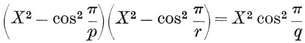 x=2 cos ξ1, 2 cos ξ2
 . By analogy with the three-dimensional case, we let h denote the period of the double rotation R1 R2 R3 R4. The details are as follows :
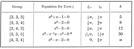
When n>4, we make use of the Chebyshev polynomials135
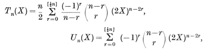
or 136
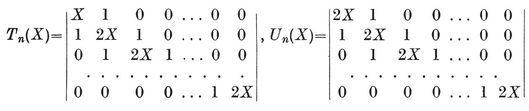
In the case of the symmetric group [3*n*–1], the equation 12·33 (with every row of the determinant doubled) becomes
Un(X)=0.
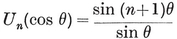 ξk are the values of 2θ for which sin (n+1)θ
Thus the period of R1 R2 . . . R*n* is n+1, in agreement with the representation of the reflections as transpositions :
R1 = (12), R2 = (2 3), . . . , Rn = (n n+1).
In the case of [3*n*–2, 4] or [4, 3*n*–2
Tn(X) = 0.
Since Tn(cos θ)=cos nθ, the angles ξk are the values of 2θ for which cos nθ=0 (0< θ
Thus the period of R1 R2 . . . R*n* is 2n.
It happens that, when the ξ’s are arranged in ascending order, all of them are multiples of ξ1. Hence the period of R1 R2 . . . R*n* is always 2π/ξ1 greatest[image]
[image]{.image .placeholder original-image-src=“content/images/00114” original-image-title=“” width=“0in” height=“0in”} {p, q, . . . , ω[image]{.image .placeholder original-image-src=“content/images/00114” original-image-title=“” width=“0in” height=“0in”}p, q] takes us one step along a Petrie polygon of the regular polyhedron or tessellation {p, q}, and that the product of the four generating reflections of [4, 3, 4] has a similar effect on the regular honeycomb {4, 3, 4}. We proceed to generalize these results to n dimensions.
We recall that a Petrie polygon of {p, q[image]{.image .placeholder original-image-src=“content/images/00114” original-image-title=“” width=“0in” height=“0in”}p, q, r} as a skew polygon such that any three consecutive sides, but no four, belong to a Petrie polygon of a cell. Finally, a Petrie polygon of an n-dimensional polytope, or of an (*n–*1)-*dimensional honeycomb, is a skew polygon such that any n–*1 consecutive sides, but no n, belong to a Petrie polygon of a cell. This, of course, is an inductive definition. We might have begun by declaring that the Petrie polygon of a plane polygon is that polygon itself. Moreover, instead of “ n−1 consecutive sides” we could have said “ n consecutive vertices ”, and instead of a polytope we may consider the corresponding spherical honeycomb.
Let A–1 A0 A1 . . . A*n*–2 A*n*–1 . . . be a Petrie polygon of the spherical or Euclidean honeycomb {p, q, . . . , ω}, so that A–1 A0 A1 . . . A*n*–2 and (say) B A0 A1 . . . A*n*–2 A*n*–1 belong to Petrie polygons of two adjacent cells. Choose the orthoscheme P0 P1 . . . P*n*–1 in such a position that P0 is A0, P1 is the mid-point of A0 A1, and P*k* is the centre of the k-dimensional element A0 . . . A*k. Let R*k*+1 denote the reflection opposite to Pk* (i.e., the reflection in the hyperplane containing all the P’s except P*k). We shall find that the operation R1 R2 . . . Rn[image]{.image .placeholder original-image-src=“content/images/00114” original-image-title=“” width=“0in” height=“0in”}permutes the vertices of the Petrie polygon. Actually they are shifted backwards; it is the inverse operation Rn* . . . R2 R1 that shifts them forwards, transforming A*j* into A*j*+1 for every j. In fact, we shall prove that
[image]

This transformation of spherical or Euclidean (n–1)-space is completely determined by its effect on the n points A–1, A0, . . . , A*n*–2 ; so the restriction “j ≤*n–*2 ” can afterwards be removed.
When n=2 we have a plane polygon A0A1 . . . ; P0 is another name for A0, and P1 is the mid-point of the arc A0 A1 of the circum-circle. R1 and R2 are the reflections in P1 and P0 (or in the radii to these points), so R2 R1 is the rotation from A0 to A1**,** as in Fig. 12.4A.
When n=3 we have a plane or spherical tessellation such as Fig. 5.9A (on page 90), but with K, M, O, Q re-named A2, A1, A0, A–1 (as in Fig. 12.4B), so that A–1 A0 A1 and B A0 A1 A2 are two adjacent faces. The rotation R2 R1 about P2 transforms B into A0, A0 into A1, and A1 into A2. Hence

When n=4 we have the situation illustrated in Fig. 5.9B, but with L, M, N, O, P re-named A3, A2, A1, A0, A–1.
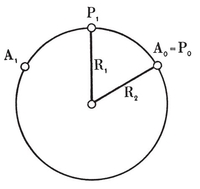
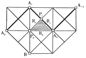
We prove the general case by induction, assuming the result for an (n–1)-dimensional polytope, such as the cell B A0 . . . A*n*–1 of the given honeycomb. Thus we assume that R*n*–1 . . . R2 R1 transforms B into A0, A0 into A1, . . . , and A*n*–2 into A*n*–1. Now Rn, being the reflection in the hyperplane A0 A1 . . . A*n*–2, transforms the cell B A0 A1 . . . A*n*–2 into the adjacent cell A–1 A0 A1 . . . A*n*–2. Hence
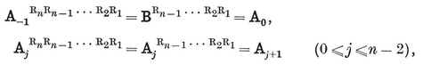
[image]
Thus the Petrie polygon of { p*,* q*,* r*, … ,* w*}* is a skew h-gon, where is the greatest root of the equation
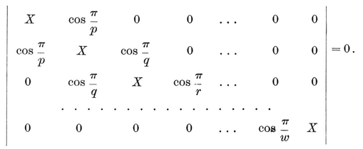
In particular, the Petrie polygon of {3, 4, 3} is a skew dodecagon, and the Petrie polygons of {3, 3, 5} and {5, 3, 3} are skew triacontagons. (See the table on page 221.) Since 1 for αn, and h=2n for βn, the Petrie polygons of these simplest polytopes include all the vertices of each.
[image]{.image .placeholder original-image-src=“content/images/00114” original-image-title=“” width=“0in” height=“0in”}[image]{.image .placeholder original-image-src=“content/images/00114” original-image-title=“” width=“0in” height=“0in”}p, q] to contain the central inversion, i.e., for the polyhedron {p, qp, q, . . . , w], or the number of sides of the Petrie polygon of {p, q, . . . , w}.
The odd polygons {p} (p odd) and simplexes an (n> 1) are certainly not centrally symmetrical ; for they have vertices opposite to cells. Hence their symmetry groups, [p] (p odd) and [3n-1] (n> 1), do not contain the central inversion. We proceed to prove that all the other finite groups [p, q, . . . , w] do contain the central inversion, in the form
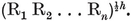
We have seen that the orthogonal transformation R1 R2 . . .R*n* n is odd. Moreover, ξ11 say

, all integers).
It follows that, when h mj *π;*combined, when n
(i) h must be even ;
(ii) every mj must be odd ;
(iii) when n
The following table shows that these conditions are satisfied in each case :
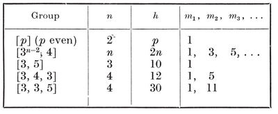
Thus all regular polytopes are centrally symmetrical, except the odd polygons and the simplexes (n≥2)
[image]{.image .placeholder original-image-src=“content/images/00114” original-image-title=“” width=“0in” height=“0in”} Knowing which regular polytopes are centrally symmetrical, we can easily find how many hyperplanes of symmetry each one has.
An odd polygon {p} obviously has N1=p lines of symmetry, namely the perpendicular bisectors of its sides. Similarly, the simplex an A0 A1 . . .A*n* is generated by the transpositions
R1 = (A0 A1), R2 = (A1 A2), . . . , R*n* = (A*n*−1 A*n*),
each of which is the reflection in the hyperplane joining the mid-point of an edge to the opposite αn−2; and all[image]{.image .placeholder original-image-src=“content/images/00114” original-image-title=“” width=“0in” height=“0in”}n dimensions). In other words, [3*n*−1] is the symmetric group of degree n
n.*n*−1*n*−1 *n*−2*n*−2 is centrally symmetrical. Reciprocally, there is a reflection for each pair of opposite vertices provided the vertex figure is centrally symmetrical, and a reflection for each pair of opposite edges provided the “ second vertex figure ” is centrally symmetrical. These remarks enable us to tabulate the number of hyperplanes of symmetry in each case, as follows :
¶ –
For instance, the above entry for βn means that there are n reflections interchanging pairs of opposite vertices, and n(n−1) interchanging pairs of opposite edges. (There is no reflection interchanging a pair of opposite αk’s for k>1, as such ak’s[image]{.image .placeholder original-image-src=“content/images/00114” original-image-title=“” width=“0in” height=“0in”}p] (p even), [3*n*−2, 4], and [3, 4, 3] have each two types of reflection, while [3, 5] and [3, 3, 5] have each only one. Hence the above list is complete.
It is remarkable that all these cases are covered by one simple formula :
[image]{.image .placeholder original-image-src=“content/images/00114” original-image-title=“” width=“0in” height=“0in”}. The symmetry group of an n-dimensional regular polytope containsreflections.
The case when n[image]{.image .placeholder original-image-src=“content/images/00114” original-image-title=“” width=“0in” height=“0in”}n. As an interesting consequence of the case when n = 4, we shall obtain an algebraic expression for gp, q, r in terms of p, q, r, and h.
[image]{.image .placeholder original-image-src=“content/images/00114” original-image-title=“” width=“0in” height=“0in”}[image]{.image .placeholder original-image-src=“content/images/00114” original-image-title=“” width=“0in” height=“0in”}p, q equators of the simplicially subdivided spherical tessellation {p, q}. This “ simplicial subdivision” is the arrangement of g = gp,*q* right-angled spherical triangles into which the sphere is decomposed by the planes of symmetry of the solid. The great circles that lie in these planes were formerly called “ lines of symmetry,” but perhaps a more vivid name is reflecting circles. Typical equators appear in Figs. 4.5A and B as broken lines, each penetrating a cycle of 2h triangles. (See also Fig. 12.7A, where the case p = q = 3 is shown in stereographic projection.) Since the arc of an equator that lies inside one of the triangles is the “ altitude line ” perpendicular to the hypotenuse from the opposite vertex, each triangle in the cycle is derived from one of its neighbours by the reflection R2 in their common hypotenuse 02, and from the other one by the half-turn R3R1 about their common vertex 1 (where two reflecting circles cross each other at right angles). The product of these two transformations is the rotatory reflection R2R3R1, which transforms each triangle into the next but one. Since R1R2R3 is conjugate to R2R3R1, we thus verify again that its period is h. Since each equator penetrates 2h of the g triangles, the number of equators is g/2h.
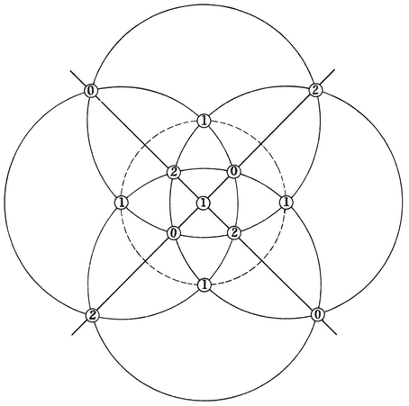
As we saw at the end of page 67, the reflecting circles can be counted by considering the h pairs of antipodal points in which they intersect a single equator (the broken line in Fig. 12.7A). Some such points are of type 1 ; others lie on arcs 02. Since they occur alternately, there are h of either kind. Each point 1 belongs to two orthogonal reflecting circles, and each point of the other kind belongs to just one. Hence the total number of reflecting circles is 3h/2.
The analogous simplicial subdivision of the spherical honeycomb {p, q, r} consists of the g = gp, *q,* *r* tetrahedra 0123 into which a hypersphere (in Euclidean 4-space) is decomposed by the hyperplanes of symmetry of the polytope {p, q, r}. The great spheres that lie in these hyperplanes are naturally called reflecting spheres. As before, we let R*k*+1 denote the reflection in the face of 0123 opposite to the vertex k. Instead of a triangle 012 with its hypotenuse 02 and opposite vertex 1 (where the right angle occurs), we now use a quadrirectangular tetrahedron 0123 and concentrate our attention on two opposite edges 02 and 13, at each of which the dihedral angle is a right angle. The product of half-turns about these two opposite edges, namely
R2R4[image]{.image .placeholder original-image-src=“content/images/00114” original-image-title=“” width=“0in” height=“0in”}1R3 = R2R1R4R3,
being conjugate to R4R3R2R1, is of period h = hp, q. r. Applying either half-turn to the initial tetrahedron, we obtain another tetrahedron sharing with it an edge at which the faces are orthogonal. Each new tetrahedron has an opposite edge around which we can make another half-turn. Continuing in this manner we obtain a cycle of 2h tetrahedra, adjacent pairs of which share such an edge.
Returning to the initial tetrahedron 0123, we observe that the edges 02 and 13 are arcs of two great circles which, being skew, have two common perpendiculars (themselves great circles). These common perpendiculars are preserved by both half-turns and so also by their product R2R1R4R3. Hence they are the two axes of this double rotation ; and the two distances between the great circles 02 and 13equator along which the 2h tetrahedra are strung like beads on a necklace, or like a “ rotating ring of tetrahedra ” (Ball 1, p. 153, where, however, the tetrahedra were tacitly assumed to be regular, except in the footnote).
The analogous arrangement in the Euclidean honeycomb {4, 3, 4} is an infinite sequence of tetrahedra 0123 whose opposite edges 02 and 13 are generators of a helicoid. (See Fig. 12.7B
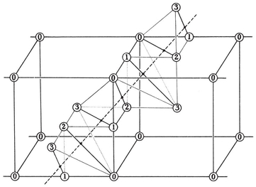
To count the reflecting spheres, we consider the pairs of antipodal points in which they intersect a single equator. Each point of this kind belongs either to one of the h edges 02 or to one of the h edges 13. In either case, the edge belongs to two orthogonal spheres. Hence the total number of spheres is
2h*.*
When n, > 4, the analogous conclusion is that opposite elements 024 . . . and 135 . . . of any one of the g characteristic simplexes 0123 . . . have a common perpendicular (great circle) which measures the absolutely shortest distance between them. This equator is transformed into itself by each of two congruent transformations of period 2 : the product R2R4R6024. . . , and the product R1R3R5 135 . . . . Applying these two transformations to the simplex 0123 . . . , we obtain its two neighbours, one before and one after, in a necklace of hypersolid beads strung along the equator. The number of beads in the whole necklace, being twice the period of the product
[image]
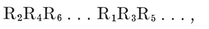
is 2h. For, this product is conjugate to R1R2 . . . R*n* (Coxeter 5, p. 602). The kind of manipulation that is needed in the proof will become clear from the following details of the case when n = 6. Writing “~” for “ which is conjugate to,” and remembering that R*k* is commutative with all the other R’s except R*k*±1, we have
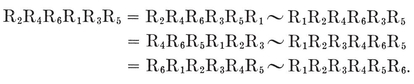
Each reflecting hypersphere intersects this equator in a pair of antipodal points. Such a point belongs either to one of the h elements 024 . . . or to one of the h elements 135

[image]{.image .placeholder original-image-src=“content/images/00114” original-image-title=“” width=“0in” height=“0in”}proved, whereas on page 227 it was merely verified.
Since each equator penetrates 2h of the g characteristic simplexes, there are altogether g/2h equators. To count the (n − 2)-dimensional simplexes into which one reflecting hypersphere is dissected by all the others, we observe that each equator meets the reflecting hypersphere in a pair of antipodal points lying on elements 024 … or 135. . . . Hence the desired number of (n − 2)-dimensional simplexes (each possessing either an element 024 . . . or an element 135 … , but not both) is equal to twice the number of equators, namely
g/h.
Since each of the ng bounding cells of the g characteristic simplexes occurs twice in the list of all the (n[image]

[image]{.image .placeholder original-image-src=“content/images/00114” original-image-title=“” width=“0in” height=“0in”}g in four dimensions. In the four-dimensional case, the total area of the 2h reflecting spheres is 8πh. Since these great spheres decompose the hypersphere into the g characteristic tetrahedra, their total area is also equal to the sum of the angular excesses of 2g spherical triangles, each occurring twice among the 4g faces of the g characteristic tetrahedra. Since the sum of all the angles of all the triangles is g/[image]
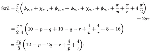
whence
[image]
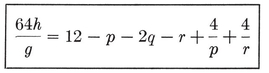
This is the formula which was promised on pages 133, 209, and 227. Since cos π[image]{.image .placeholder original-image-src=“content/images/00114” original-image-title=“” width=“0in” height=“0in”}h/g is actually a trigonometrical formula for g. It is thus “ elementary,” in contrast to Schläfli’s expression
(see page 142). Moreover, it is very easy to use ; e.g., since h3,3,5 = 30,
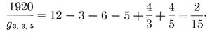
It may be regarded as the four-dimensional analogue of
The five-dimensional analogue,137
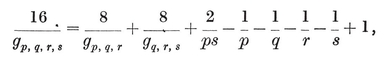
[image]
N0 − N1 + N2 − N3 + N4 = 2.
[image]{.image .placeholder original-image-src=“content/images/00114” original-image-title=“” width=“0in” height=“0in”}gp,q,r,s as a trigonometrical function of p, q, r, s.
[image]{.image .placeholder original-image-src=“content/images/00114” original-image-title=“” width=“0in” height=“0in”}[image]{.image .placeholder original-image-src=“content/images/00114” original-image-title=“” width=“0in” height=“0in”}1[image]{.image .placeholder original-image-src=“content/images/00114” original-image-title=“” width=“0in” height=“0in”}P0P2 and P1P3
[image]{.image .placeholder original-image-src=“content/images/00114” original-image-title=“” width=“0in” height=“0in”}11 ; Steinberg 2). Thus the products of generators of the trigonal groups (see page 204) work out as follows :
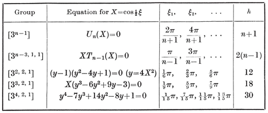
Here, as before, h[image]{.image .placeholder original-image-src=“content/images/00114” original-image-title=“” width=“0in” height=“0in”}*n*−3, 1, 1] (n even), [33, 2, 1] and [34, 2, 1] all contain the central inversion, while [3*n*−3, 1, 1] (n odd) and [32, 2, 1[image]
1 + y1 + y2 + . . .+ yn
is equal to h.
In the First Edition, this page ended with an appeal for some reader to supply a direct proof “ that the number of reflections (when n = 4) cannot be less than 2h.[image]{.image .placeholder original-image-src=“content/images/00114” original-image-title=“” width=“0in” height=“0in”}1R2 . . . R*n*[image]{.image .placeholder original-image-src=“content/images/00114” original-image-title=“” width=“0in” height=“0in”}n = 3 but for all values of n.
It seems fitting to close this chapter with a few words about the life of Pieter Hendrik Schoute. He was born in 1846 at Wormerveer, Holland. He started his career as a civil engineer, but in 1870 took his Ph.D. at Leiden with a dissertation on “ Homography applied to the theory of quadric surfaces ”. After eleven years of teaching he became a professor of mathematics at Groningen, where he worked until his death in 1913. His uninterrupted series of mathematical papers (including some thirty on polytopes) began in 1878. The work on congruent transformations appeared in 1891, and from that time he became increasingly interested in n-dimensional Euclidean geometry. About 1900 H. Schubert asked him to write a couple of volumes for his Sammlung mathematischer Lehrbiicher (Schoute 4 and 6). Die linearen Räume appeared in 1902, and Die Polytope in 1905 ; they are still “ classics ”, though by no means easy to read.
[]
¶ CHAPTER XIII
SECTIONS AND PROJECTIONS
THIS chapter provides some indication of the manner in which the more complicated illustrations in this book were constructed. The illustrations make no important contribution to the theoretical development of our subject, but they have a psychological value in making us feel more familiar with the individual polytopes. It may be claimed, also, that they have some artistic merit.
Inhabitants of Flatland,138 desiring to get an idea of solid figures, would have two general methods available to them : section and projection. According to the first method, they would imagine the solid figure gradually penetrating their two-dimensional world, and consider its successive sections; 139e.g., the sections of a cube, beginning with a vertex, would be equilateral triangles of increasing size, then alternate-sided hexagons (“ truncated ” triangles), and finally equilateral triangles of decreasing size, ending with a single point—the opposite vertex. According to the second method, they would study the shadow of the solid figure in various positions ; e.g., a cube in one position appears as a square, in another as a hexagon.
[image]{.image .placeholder original-image-src=“content/images/00114” original-image-title=“” width=“0in” height=“0in”}n[image]{.image .placeholder original-image-src=“content/images/00114” original-image-title=“” width=“0in” height=“0in”}γn onto a three-space are found to be zonohedra.
It is perhaps worth while to mention a third method for representing an n-dimensional polytope in n−1 dimensions: the unfolded “ net ”. Two instances will suffice. The cube γ3 is unfolded into a kind of cross, consisting of a square with four other squares attached to its respective sides and a sixth beyond one of those four. The hyper-cube γ4 is unfolded into a kind of double cross, consisting of a cube with six other cubes attached to its respective faces and an eighth beyond one of those six. But we shall not have occasion to use this method.
[image]{.image .placeholder original-image-src=“content/images/00114” original-image-title=“” width=“0in” height=“0in”} The Flatlander’s sequence of parallel sections of a regular solid might be taken in any direction, but it would be simplest to use planes perpendicular to one of the axes of symmetry O*j* O3, which join a vertex (j=0) or mid-edge point (j=1) or face-centre (j=2) to the centre of the solid. Analogously, we three-dimensional creatures can get some idea of the appearance of the four-dimensional regular polytopes by observing a sequence of parallel “ solid sections ”, perpendicular to one of the four principal directions O*j* O4(j=0, 1, 2, 3). For the sake of completeness, we shall describe the nn by a sequence of parallel hyperplanes perpendicular to the line O*j* O*njnj* itself.
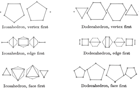
n. Each section is, of course, a convex (nnn) determine an inscribed polytope which we shall call a simplified section. Fig. 13.1A140 shows the sections of the icosahedron and dodecahedron (n=3), with the simplified section drawn in full lines, and the rest of the section (when there is any more) in broken lines. To obtain the simplified sections ab initio[image]{.image .placeholder original-image-src=“content/images/00114” original-image-title=“” width=“0in” height=“0in”}n in sets of parallel hyperplanes perpendicular to O*j* O*n.*
When n>3 we shall be content to describe those sequences of sections which begin with a vertex or a cell, so that j=0 or n−1. The simplified sections beginning with a vertex are conveniently denoted by
O0, 10, 20, . . , k0
(so that 00 is the vertex itself, and 10 is similar to the vertex figure), and those beginning with a cell by
1*n*−1, 2*n*−1, . . .
(so that 1*n*−1is the cell itself). In the case of αnn has central symmetry. Then the last section in each sequence will be the same figure as the first, the last but one the same as the second, and so on ; thus (k−i)0 and i0 are alike, and k0 is the vertex opposite to 00.
[image]{.image .placeholder original-image-src=“content/images/00114” original-image-title=“” width=“0in” height=“0in”}corresponding sections 1*n*−1, 2*n*−1, . . . : the numbers of vertices are proportional, and so are the circum-radii. As a trivial instance, all the vertices of either βn or γn are included in the two sections 1*n*−1 and 2*n*−1, which are two opposite cells.
In tabulating the simplified sections i0, it is convenient to let a denote the distance from the point 00 to any vertex of i0n as unit ; e.g., α=1 for 10, 0R/l for the “ antipodes ” k0, and 1R/l for (k−1)0. In other words, the edge length being 2l, the vertices of i0 are distant 2la from O0.
The simplified section i0 may be a regular polytope of edge 2lb (say), or it may be irregular. In the latter case we shall be interested in the possible occurrence of inscribed regular polytopes (having some of the same vertices) ; e.g., the section 20 or 30[image]
In the case of the cross polytope βn, 20 is the vertex opposite to 00, while 10 is the equatorial βn−1 (with a=b=1).
We saw, in [image]{.image .placeholder original-image-src=“content/images/00114” original-image-title=“” width=“0in” height=“0in”} that the vertices of the measure polytope γn are
( ± 1, ± 1, . . . , ± 1, ± 1).
Shifting the origin to (−1, −1, . . . , −1, −1), and doubling the unit of measurement, we obtain
13·11
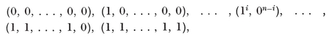
with the coordinates permuted arbitrarily. Here the 2n** vertices have been distributed into sets of
which belong to the respective sections
0**0, 10, . . . , i0, . . . ,** (n − 1)0, no.
Hence, by 8·76,
(with α=√i, b=√2) ; e.g., the section 20 of γ4
For the remaining regular polytopes in four dimensions, we express the coordinates of the vertices of II4 in such a form that the line O4 O0 or O4 O3 may be taken along the x4-axis. Then the simplified sections are picked out by arranging the vertices of II4 according to decreasing values of x4 ; and in each case the values of (x1, x2, x3) enable us to ascertain the shape of the simplified section (which is an ordinary polyhedron).
The {3, 4, 3} with vertices 8·71 and 8·73 can be derived from its reciprocal, 8·72, by the transformation
x1′ = x1 − x2 , x2′ = x1 + x2, x3′ = x3 − x4, x4′ = x3 + x4,
which is a Clifford displacement (page 217) combined with a magnification. Applying the same transformation to the {3, 3, 5} with vertices 8·71, 8·73, 8·74, we obtain the vertices of another {3, 3, 5} (of edge 2τ-1√2)141 as the permutations of (τ2, τ−1, τ−1, τ−1) and (τ, τ, τ, τ-2) with an even number of minus signs, (√5, 1, 1, 1) with an odd number of minus signs, and (±2, ±2, 0, 0).
Similarly, the reciprocal {5, 3, 3} (of edge 2τ−2√2) is given by the permutations of
¶ –
and ( ± 4, 0, 0, 0), ( ± 2, ± 2, ± 2, ± 2), ( ± 2τ, ± 2, ± 2τ−1
Using these results, and referring to § 3·7, we obtain the sections exhibited in Table V (pages 298-301). The latter half of Table V (v) has been omitted, to save space; but nothing is lost, as (30−i)0 is just like i0, and the value of α is given in the final column. Most of the sections of {5, 3, 3} are irregular, but some (viz., 30, 80, 110, 120, 150) are partially regular, in the sense that their vertices include the vertices of one or more regular solids. The pairs of interpenetrating icosahedra in the two similar sections 30 and 110 are evident from 3·75 (since all permutations of the three coordinates occur, whereas the cyclic permutations give an icosahedron). The reciprocal pair of interpenetrating dodecahedra 142 occurs in 80. Here the two dodecahedra (one given by cyclic permutations of the given coordinates) have eight common vertices (±2, ±2, ±2), belonging to one of the five cubes that can be inscribed in either dodecahedron. The remaining eight cubes of the two {5, 3} [5{4, 3}]’s form a symmetrical set ; each of the 8 + 24 vertices belongs to two of them. In other words, 80 contains a set of 1 + 8 cubes (one special). Reciprocating again, we obtain a set of 1+8 octahedra, as in 150. By 3·77, the same vertices belong to two interpenetrating icosidodecahedra, whose common vertices are those of the special octahedron. The remaining 48 vertices of the two icosidodecahedra are distributed among the remaining 8 octahedra. Finally, the connection between 150 and 30 (or 110) is as follows : the two overlapping compounds [5{3, 4}]{3, 5} in 150 have the same face-planes as a pair of icosahedra like 30 or 110.
13·2. Orthogonal projection onto a hyperplane. The general procedure for projecting an n-dimensional figure may be described as follows. Given an s-space and an (n−s)-space which have only one common point (and therefore “ span ” the whole n-space), we project onto the s-space by drawing, through each point of the figure, an (n−s)-space parallel to the given (n−s)-space, to meet the s-space in a definite “image” point. This process of parallel projection is called orthogonal projection if the (n−s)-space is completely orthogonal to the s-space.
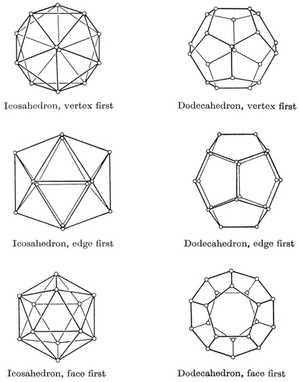
The most familiar instance of parallel projection (with n=3 and s=2) occurs when the sun casts a shadow on the ground. The projection is orthogonal if the sun is at the zenith. Fig. 13.2A shows various orthogonal projections of the icosahedron and dodecahedron (i.e., shadows of wire models of the vertices and edges). Comparing this with Fig. 13.1A, we see how such a projection can be derived from a sequence of sections. Each section is projected (onto a parallel plane) without any distortion ; so the whole projection can be constructed by superposing the simplified sections and joining certain pairs of vertices (by foreshortened edges).
In the case of the “ vertex first ” projection, two opposite vertices would naturally be projected into coincidence at the centre of the plane figure. In Fig. 13.2A we have avoided this coincidence by making a slight distortion. We may justify this distortion by pretending that the direction in which we project differs from the direction O3 O0 by a very small angle. A similar device has been employed to separate two opposite edges in the “ edge first ” projection. To save space we have omitted the analogous figures for the simpler Platonic solids ; but it is worth while to mention that the neatest way to separate the nearest and farthest faces of the cube in its “ face first ” projection is to introduce a slight degree of perspective, making the one face a little smaller than the other. (The result, in this case, is a Schlegel diagram ; cf. page 10.)
n can be superposed concentrically, in their proper size and orientation, to form an (n−1)-dimensional projection. The only case of practical interest is when n4’s have been made by Donchian, using straight pieces of wire for the edges, and globules of solder for the vertices. (See Plates IV-VIII.) The vertices are distributed on a set of concentric spheres (not appearing in the model), one for each pair of opposite sections. Donchian did not attempt to indicate the faces, because any kind of substantial faces would hide other parts (so that the model could only be apprehended by a four-dimensional being). The cells appear as “ skeletons ”, usually somewhat flattened by foreshortening but still recognizable. Parts that would fall into coincidence have been artificially separated by slightly altering the direction of projection, or introducing a trace of perspective.
The “ vertex first ” and “ cell first ” projections of {3, 3, 5} are shown in Plate IV (facing page 160) and again in Plate VII (page 256). The “ cell first ” projection of {5, 3, 3} is shown in Plate V (page 176) and again in Plate VIII (page 273).
PLATE VI
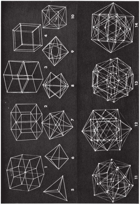
PROJECTIONS OF THE SIMPLER HYPER SOLIDS
The arrangement of figures in Plate VI is as follows :
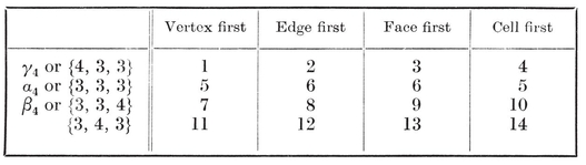
Some of these figures are quite easy to describe. Fig. 5 is a tetrahedron with all its vertices joined to its centre ; Fig. 10 is a cube with its face-diagonals drawn ; and Fig. 14 is a cuboctahedron with its vertices joined to pairs of points near the centres of its square faces.
Donchian claims, with some justification, that these models are more perspicuous than those of Schlegel 2, which are exhibited in certain museums. Donchian’s are more like portraits, involving a minimum of distortion. As he says, “ They help to remove the mystery from a seemingly complicated subject… Each component part is distinctly visible and tangible, in practically its true position and relationship.”
13⋅3. Plane projections of αn, βn, γn. In Figs. 7.2A, B, C, we assumed that the vertices of α4 and β4 can be projected into the vertices of the regular pentagon {5} and octagon {8}, and that γ4 can be projected isometrically (so that all the edges project into equal segments). One feels instinctively that such highly symmetrical figures are really orthogonal projections. We shall find that this instinctive feeling is in fact justified.
n] completely orthogonal planes, along with a reflection when n is odd. We saw also that one of the angles of rotation is 2π/h, while the rest are multiples of that one, say 2mπ/h for various values of m. (See the table in § 12⋅5.) It follows that the orthogonal projections of the Petrie polygon on the various planes are regular polygons {h/m}, with m= 1 in one case.
When m= 1, so that the Petrie polygon projects into an ordinary regular h-gon, it is not surprising to find that the remaining vertices and edges of the polytope project into points and segments inside the h-gon. (See Figs. 2.6A, 7⋅2A, B, C, 8⋅2A, 13⋅3A, and the frontispiece.) In other words, the h-gon is the periphery of the projection, like the shadow of an opaque solid.
When the polytope is αn or βn, all its vertices belong to one Petrie polygon, and therefore every edge is either a side or a diagonal of that skew polygon. Hence the vertices and edges of αn can be projected into an {n+1} with all its diagonals, while the vertices and edges of βn can be projected into a {2n) with all its diagonals except those that pass through the centre.
The corresponding projection of γn is isometric ; for every edge of γn is parallel to one of the diameters of the reciprocal βn, and these project into the diameters of the {2n}, which are all equal. The coordinates 13⋅11 (on page 239) show clearly that any vertex
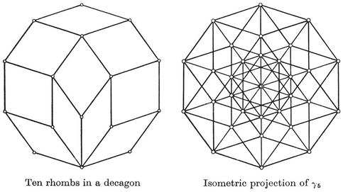
can be derived from a particular vertex by applying a vector of the form
13⋅31

where the e’s are selected from n unit vectors in perpendicular directions. In particular, the vectors e1; e2, . . . , en proceed along n consecutive sides of a Petrie polygon (with −e1, −e2, . . . , −en along the remaining n sides). We know that there is one plane on which this skew polygon projects into an ordinary {2n}. Then the vectors ej project into vectors along n consecutive sides of this {2n}. The projections of the remaining vertices and edges may be constructed by filling the {2n n=4 and n=5 are shown in Figs. 7.2C and 13⋅3A, respectively.
13⋅4. New coordinates for αn and βn. We found, on page 222, that the angles of rotation of the Petrie polygons for an and βnnn] odd multiples of π/n, respectively. This remark suggests a new representation for these polytopes in terms of Cartesian coordinates.
Let A*k* denote the point (x1, . . . , xn), where
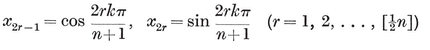
and if n is odd, xn = (−1)k/√2. Then, if 0 < k < n + 1*,* we have
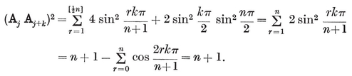
Hence A0 A1 . . . A*n*
Again, let B*k* denote the point (x1, … , xn), where
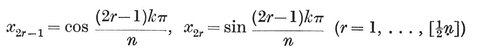
and if n is odd, xn = ( − 1)k/√2. Then, provided k is not divisible by n,
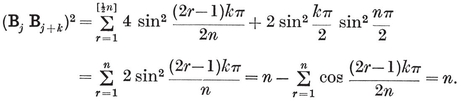
Hence B1 … B2*n* is a cross polytope of edge √n.
We obtain the orthogonal projections, {n+1} and {2n}, by keeping the coordinates x1, x2, and discarding all the rest.
13⋅5. The dodecagonal projection of {3, 4, 3}. Other polytopes may be treated similarly. The 24-cell {3, 4, 3} has a Petrie polygon A0 A2 A4 . . . A22, where A*k* (k even) is
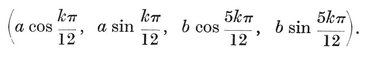
Since the triangle A0 A2 A4 is equilateral,
Thus, if the circum-radius is 1, so that the edge also is 1, we have
13⋅51

In other words, a and b are the positive roots of the equation
6x4 − 6x2 + 1 = 0 .
Now, A0 A2 A4 A6 is part of the Petrie polygon of an octahedron, which has an equatorial square A0 A4 A6 B1, where B1 is
or
This is one of twelve vertices B1 B3 B5 … B23, where Bk** (k odd) is
The 24 vertices of {3, 4, 3} consist of the twelve A’s and the twelve B’s. The 96 edges are :
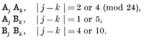
In other words, there are 12 like A0 A2, 12 like A0 A4, 24 like A0 B1 (and A2 B1), 24 like A0 B5 (and A6 B1), 12 like B1 B5, and 12 like B1 B11. As for the 24 cells (octahedra), there are 12 like A0 A2 A4 A6 B5 B1 and 12 like B1 Bn B21 B7 A2 A6. (See Fig. 13.5A.) The twelve B’s, taken in the order
13⋅52
B1 B11 B21 B7 B17 B3 B13 B23 B9 B19 B5 B15,
form another Petrie polygon.
After projection onto the (x1, x2)-plane, the A’s and B’s form two concentric dodecagons, inscribed in circles of radii a and b.
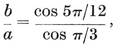
the chord **A0 A10**π) contains the chord B1 B9Fig. 8.2A (on page 149) is quite easy to draw : within the dodecagon A0 A2 … A22 (Fig. 13.5B) we locate B1 as the point where A0 A10 meets A2 A16. Triangles like A0 A2 B1, and squares like A2 A4 B5 B1, are projected without distortion.
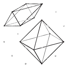
Two cells of
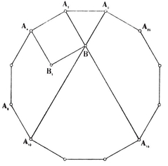
How to locate the B’s
13⋅6. The triacontagonal projection of {3, 3, 5}. More complicated considerations of the same kind give us the 120 vertices of the 600-cell {3, 3, 5} in the form
A0 A2 . . . A58, B1 B3 . . . B59, C1 C3 . . . C59, D0 D2 . . . D58,
where, in terms of θ=π/30=6°,
A*k* (k even) is (a cos kθ, a sin kθ, d cos 11 kθ, d sin 11 kθ),
B*k* (k odd) is (b cos kθ, b sin kθ, c cos 11 kθ, c sin 11 kθ),
C*k* (k odd) is (c cos kθ, c sin kθ, −b cos 11 kθ, −b sin 11 kθ),
D*k* (k even) is (d cos kθ, d sin kθ, −a cos 11 kθ, −a sin 11 kθ).
The numbers a, b, c, d are connected in various ways, such as
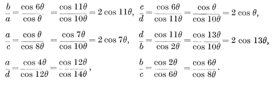
If the circum-radius is 1, so that the edge is τ-1, we have
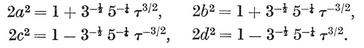
In other words, a, b, c, d are the positive roots of the equation
45x8 − 90x6 + 60x4 − 15x2 + 1 = 0.
The 720 edges are :
¶ –
Thus A0 A2 . . . A58 and
13⋅61
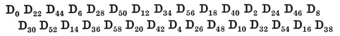
are Petrie polygons.
The various types of cell are all given by taking sets of four consecutive vertices of two further Petrie polygons :
13⋅62
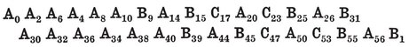
and
13⋅63
(Fig. 13.6A). Thus the 600 tetrahedra consist of thirty of each of the “ symmetrical ” types
AAAA**,** AABB**,** CCDD**,** DDDD
and sixty of each of the “ asymmetrical ” types
AAAB**,** AABC**,** ABBC**,** ABCC**,** BBCD**,** BCCD**,** BCDD**,** CDDD**.**
(For instance, we regard A4 A8 A10 B9 as being of the same type as A6 A2 A0 B1, since either can be derived from the other by subtracting respective suffixes from 10.)
After projection onto the (x1, x2)-plane, the A’s, B’s, C’s, and D’s form four concentric triacontagons, inscribed in circles of radii a, b, c, and d. There is no need to compute these magnitudes ;
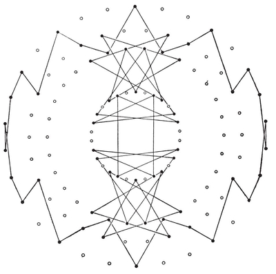
Two Petrie polygons of
for, when we have drawn the outermost triacontagon A0 A2 … A58 (Fig. 13.6B), the relations
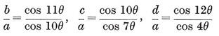
enable us to locate B1, C1, Do as the respective points of intersection
(A2 A40 ⋅ A22 A0), (A4 A44 ⋅ A18 A58), (A8 A44 · A16 A52).
The vertices of the reciprocal {5, 3, 3}, being the centres of the 600 cells of {3, 3, 5}, project into the centroids of the projected sets of four points, e.g., A0 A2 A4 A6. We thus have a plane figure in which 600 points occur on twelve concentric circles : thirty on each of four circles (including the outermost), and sixty on each of the remaining eight. Such a drawing has been made by B. L. Chilton (Coxeter 20, p. 403).
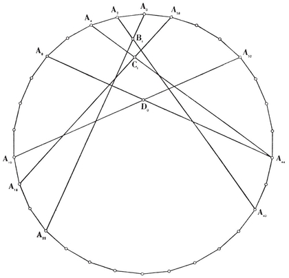
How to locate the B’s, C’s, and D’s
13⋅7. Eutactic stars. So far, we have projected polytopes of more than four dimensions into two dimensions only. It is natural to expect that a clearer idea would be obtained by projecting them into three dimensions. The simplexes an are already so simple that there is not much advantage in projecting them. (It is perhaps worth while to mention that a2p–1 can be projected into βp ; e.g., a5 into an octahedron. See Schoute 6, pp. 253-254.) But we shall describe various projections of the cross polytopes and measure polytopes.
We have seen that the vertices of βn can be orthogonally projected into the vertices of a regular 2n-gon in a suitable plane. We now ask whether they can also be projected into the vertices of a regular or quasi-regular polyhedron in a suitable 3-space. (Of course this could only happen for certain special values of n, such as 4, 6, 10. For an icosahedral projection of β6, see Schoute 6, p. 254.) There is no “ Petrie polyhedron ” to guide us in our choice of a 3-space. Nevertheless, an affirmative answer is obtained by means of the following considerations, due to Hadwiger.
We define a star (as in § 2⋅8) to be a set of 2n vectors ±a1, . . . , ±an issuing from a fixed origin in Euclidean 3-space.143 A vector s (not necessarily belonging to the star) is called a symmetry vector if the symmetry group of the star admits a subgroup under which the multiples of s are the only invariant vectors.
We define a cross to be a set of n mutually perpendicular pairs of vectors ± e1, . . . , ± en of equal magnitude, issuing from a fixed origin in Euclidean n-space. Thus the end-points of the vectors of a cross are the vertices of a cross polytope, βn. The orthogonal projection of a cross on any three-dimensional subspace is called a eutactic star. 144 If the vectors of the cross are of unit magnitude the projection is called a normalized eutactic star.
For a given set of n vectors, a1, . . . , an, we define the “ vector transformation ”
aj aj ·,
which transforms any vector x into Txaj aj · xaj · x)aj. This clearly has the properties
T(x+y)=Tx+Ty, Tλx=λTx, Tx⋅y =x· bTy,
where λ is any real number. In particular, if a1, … , an are mutually perpendicular unit vectors (in n dimensions), the n numbers aj • x are the components of x in those directions, and Tx=x. We proceed to prove Hadwiger’s principal theorem :
13⋅71. Vectors ± a*1, . . . , ± an,* in a 3-space, form a normalized eutactic star if, and only if, Tx*=*x for every x in the 3-space.145
First, given a normalized eutactic star, we shall prove that Tx=x. If n=3 the star is a cross of unit vectors, and the result is obvious. If n>3 let the given star be the orthogonal projection of a cross of unit vectors ± e1, … , ± en in an n-space containing the 3-space. Then the completely orthogonal (n—3)-space contains n vectors b1, …, bn such that
ej = aj + bj (j=1,…,n).
For all vectors x in the n-space, and in particular for such in the 3-space, we have
(ej • x)ej = x.
But, for x in the 3-space, bj • x= 0.
Hence
(aj • x)(aj + bj) = x,
and
(aj • x)bj = x−Tx.
Now, the vector on the right lies in the 3-space, while that on the left lies in the completely orthogonal (n-3)-space. Hence both vanish, and we have Tx= x.
Conversely, given a star such that Tx=x, we shall prove that it is a normalized eutactic star. If n=3 we take x to be perpendicular to two of a1, a2, a3, and deduce that it is parallel to the remaining one, i.e., that the three a’s are all perpendicular ; then taking x=ak, we deduce that ak2=1. If n> 3 we regard the 3-space as a subspace of the n-space spanned by n mutually perpendicular unit vectors p1, p2, p3, … , pn, of which the first three span the 3-space. In this n-space, consider the three vectors
qµaj • pµ)pj (µ = 1, 2, 3).
Since pj • pk = δjk, we have
qµ • qvaj • p*µ)(aj • pv) = Tpµ* • pv=pµ • pv= δµv.
Thus the three q’s are all perpendicular. Along with these, take n—3 further vectors q4, … , qn, such that
qj • qk = δjk (j, k=1, … , n).
Then any vector pqi • p)qi. Since
qµpµ • aj)pj,
we have
qµ • pkpµ • aj)δjk= pµ • ak, and
ak= (p1 p1 • + p2 p2 • + p3 p3 • )ak=(p1 q1 • + p2 q2 • + p3 q3 •)pk.
So, if we define
bk = (p4 q4 • + … +pn qn • )pk and ek = ak + bkpi qi • pk,
we have
ej • ekqi • pj)(qi • pk) = pj • pk =δjk.
We thus express the given star as the orthogonal projection of a cross ± e1,…, ± en[image]
The effect of multiplying all the vectors a1, … , an by a number c, is to multiply Tx by c2. Hence
[image]{.image .placeholder original-image-src=“content/images/00114” original-image-title=“” width=“0in” height=“0in”}Vectors ±a1, …, ±an, in a 3-space, form a eutactic star if, and only if, Tx*=λx,* where the number λ is the same for all vectors x *(*in the 3-space).
If
(a1 a[image]{.image .placeholder original-image-src=“content/images/00114” original-image-title=“” width=“0in” height=“0in”} + …+ a*n* a*n[image]{.image .placeholder original-image-src=“content/images/00114” original-image-title=“” width=“0in” height=“0in”})x=λx* and (b1b1. + … +bm b[image]{.image .placeholder original-image-src=“content/images/00114” original-image-title=“” width=“0in” height=“0in”})x=µx,
then
(a1 a[image]{.image .placeholder original-image-src=“content/images/00114” original-image-title=“” width=“0in” height=“0in”} +… +an a[image]{.image .placeholder original-image-src=“content/images/00114” original-image-title=“” width=“0in” height=“0in”} +b1b[image]{.image .placeholder original-image-src=“content/images/00114” original-image-title=“” width=“0in” height=“0in”} +… +bmb[image]{.image .placeholder original-image-src=“content/images/00114” original-image-title=“” width=“0in” height=“0in”})x= (λ+µ)x.
Hence
[image]{.image .placeholder original-image-src=“content/images/00114” original-image-title=“” width=“0in” height=“0in”}Any two eutactic stars, with the same origin, form together a eutactic star.
The next step in our argument is the following lemma :
[image]{.image .placeholder original-image-src=“content/images/00114” original-image-title=“” width=“0in” height=“0in”}If a star ±a1, … , ±an has a symmetry vector s, then Ts is parallel to s.
PROOF. Any symmetry operation of the star, say K, permutes the n vector-pairs ± ai ; thus aiK= ± aj for some j, not necessarily different from i. This symmetry operation transforms
Txai ai · x
into
(Tx)KaiK ai[image]{.image .placeholder original-image-src=“content/images/00114” original-image-title=“” width=“0in” height=“0in”} xKaj aj[image]{.image .placeholder original-image-src=“content/images/00114” original-image-title=“” width=“0in” height=“0in”}xK =TxK.
If K belongs to the subgroup under which the multiples of s are the sole invariant vectors, then sK = s, and we deduce that (Ts)K=Ts. Thus Ts is invariant under transformation by K, which may be any operation of the subgroup. Hence Ts is a multiple of s.
We are now ready for our chief theorem :
[image]{.image .placeholder original-image-src=“content/images/00114” original-image-title=“” width=“0in” height=“0in”}A star is eutactic if its symmetry group is transitive on a set of symmetry vectors which span the 3-space.
PROOF. For each symmetry vector s, of the set considered, we have
Ts=λs
for some number λ. Since TsK=(Ts)K=λsK, λ is the same for all s’s. Since T is a linear operator, and the s’s span the 3-space, it follows that Tx=λx for every vector x. Hence the star is eutactic.
If the symmetry group is [3, 4] or [3, 5], the vectors to the vertices of the octahedron or icosahedron are symmetry vectors which span the space. Hence
[image]{.image .placeholder original-image-src=“content/images/00114” original-image-title=“” width=“0in” height=“0in”}Any star having octahedral or icosahedral symmetry is eutactic.
In particular, the vectors (from the centre) to the vertices of the octahedron, cube, cuboctahedron, icosahedron, rhombic dodecahedron, pentagonal dodecahedron, icosidodecahedron, and triacontahedron, form eutactic stars. In other words, these polyhedra are “ orthogonal shadows ” of the respective cross polytopes
β3, β4, β6, β6 again, β7, β10, β15, and β16,
The first case is trivial, since β3 is the octahedron itself. When we say that the cube is a shadow of β4, we mean that β4 projects into a cube with its interior. Two opposite cells project (without distortion) into the two regular tetrahedra inscribed in the cube, eight project into trirectangular tetrahedra (one for each corner of the cube), and the remaining six project into the faces of the cube (with their diagonals).
If the vector aj of a star has components (cj1, cj2, cj3) in terms of an orthogonal frame of reference, so that
aj = cj1 e1 + cj2 e2 + cj3 e3, eµ[image]{.image .placeholder original-image-src=“content/images/00114” original-image-title=“” width=“0in” height=“0in”}ev = δµv,
then Teµcjµ a*jcjµ* (cj1 e1 + cj2 e2 + cj3 e3[image]
[image]{.image .placeholder original-image-src=“content/images/00114” original-image-title=“” width=“0in” height=“0in”}The vectors (cj*1*, cj*2*, cj*3*) and their opposites form a normalized eutactic star if, and only if,
cjµ c*jν* = δµν (µ, ν =1, 2, 3).
When n[image]
[image]
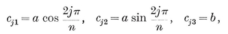
so that the vectors aj lie along n evenly spaced generators of a cone of revolution (like the ribs of an umbrella). We obtain the conditions
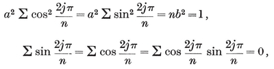
[image]
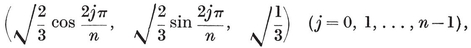
form (with their opposites) a eutactic star. Thus the cone of semi-vertical angle arc tan √2 has the remarkable property that vectors of equal magnitude, taken in both directions along n symmetrically spaced generators, form a eutactic star, for all values of n. (When n[image]{.image .placeholder original-image-src=“content/images/00114” original-image-title=“” width=“0in” height=“0in”}n/3 crosses.) In other words,
[image]{.image .placeholder original-image-src=“content/images/00114” original-image-title=“” width=“0in” height=“0in”}A right regular n-gonal prism (n even) or antiprism (n odd) is an orthogonal shadow of βn, provided its altitude is √2 times the circum-radius of its base.
When n=4 the prism is a cube, which we have already recognized as a shadow of β4. When n=5 we have a special pentagonal antiprism (with isosceles lateral faces), which is the most symmetrical projection of β5. For β6, however, we have already found two other projections which, for most purposes, are preferable to the hexagonal prism.
[image]{.image .placeholder original-image-src=“content/images/00114” original-image-title=“” width=“0in” height=“0in”}Shadows of measure polytopes[image]{.image .placeholder original-image-src=“content/images/00114” original-image-title=“” width=“0in” height=“0in”}every eutactic star determines a zonohedron which is an orthogonal shadow of γn, i.e., the surface of an orthogonal projection. In particular, since a zonohedron has the same symmetry as its star,
Every zonohedron which has octahedral or icosahedral symmetry is an orthogonal shadow of a measure polytope γn.
The number of dimensions of the measure polytope is naturally equal to the number of directions of edges of the zonohedron ; e.g., the rhombic dodecahedron is a shadow of γ4, and the triacontahedron of γ6. The fifteen equilateral zonohedra shown in Plate II (facing page 32) are shadows of γn for the following values of n :
3, 4, 6, 6, 7, 9, 10, 10, 12, 12, 12, 13, 15, 21, 24.
(The numbers in bold type refer to zonohedra having icosahedral symmetry ; the rest have octahedral symmetry.) Each 2m-gonal face (m>2) has been filled with overlapping rhombs (like Fig. 13.3A) so as to exhibit it as a plane projection (orthogonal or oblique) of an element γm. The three shadows of γ12, and the shadow of γ24, are capable of continuous variation, and any two varieties of the former may have their stars superposed to give a different shadow of γ24. But the remaining eleven (along with shadows of γ16, γ25, γ31, which have icosahedral symmetry) are unique, in the sense that no other isometric projections of the same γn can have the same symmetry. This happens because their stars are obtained by selecting one or more of the vertices 0, 1, 2 of the spherical tessellations shown in Fig. 4.5A.
By considering the star formed by equal vectors along evenly spaced generators of a cone of semi-vertical angle arc tan √2, we see that the polar zonohedra (Fig. 2.8A[image]{.image .placeholder original-image-src=“content/images/00114” original-image-title=“” width=“0in” height=“0in”}n rhombs of angle
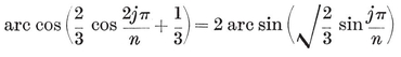
for each value of j from 1 to n−1. When n n “ vertical ” rhombs which have the same shape as the faces of the rhombic dodecahedron. When nn squares.
The isohedral rhombic icosahedron (Fig. 2.8A, n=5), whose edges make an angle arc tan τ with its axis of symmetry, is too “ oblate ” to be an orthogonal shadow of γ5 ; but this defect can be remedied by stretching it in the direction of its axis. The stretching has no visible effect on the particular projection shown in Fig. 2.8A (which is a “ plan ”) ; so I have drawn another projection (an “elevation ”) in Fig. 13.8A. This solid, bounded by ten rhombs of angle
(five at each “pole ”, shaded in the figure) and ten rhombs of angle
(in the “ tropics ”),146 is one of the most symmetrical shadows that can be found for γ[image]{.image .placeholder original-image-src=“content/images/00114” original-image-title=“” width=“0in” height=“0in”} Another is derived from the five unit vectors
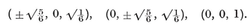
PLATE VII
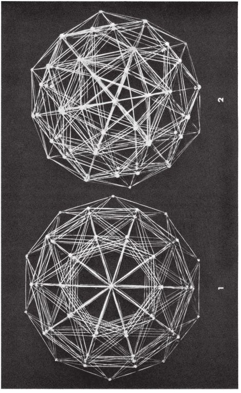
TWO PROJECTIONS OF
(See Fig. 13.8B. In this case the “ plan ” would be indistinguishable from Fig. 2.8A, n=4.) This elongated dodecahedron
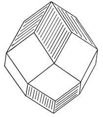
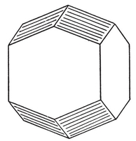
Projections of γ5
For simplicity, we have restricted consideration to projections onto a 3-space. But most of the above theory can be extended to projections onto any subspace of the n-space. For instance, the four-dimensional shadows of γn[image]{.image .placeholder original-image-src=“content/images/00114” original-image-title=“” width=“0in” height=“0in”}n segments in the star. When the zonohedron is a shadow of γn the various parallelepipeds arise as projections of elements γ3 (i.e., cubes).
[image]{.image .placeholder original-image-src=“content/images/00114” original-image-title=“” width=“0in” height=“0in”} Alicia Boole Stott (1860-1940) was the middle one of George Boole’s five daughters. Her father, who is famous for his algebra of logic and his text-book on Finite Differences, died when she was four years old ; so her mathematical ability was purely hereditary. She spent her early years, repressed and unhappy, with her maternal grandmother and great-uncle in Cork. When Alice was about thirteen the five girls were reunited with their mother (whose books reveal her as one of the pioneers of modern pedagogy) in a poor, dark, dirty, and uncomfortable lodging in London. There was no possibility of education in the ordinary sense, but Mrs. Boole’s friendship with James Hinton attracted to the house a continual stream of social crusaders and cranks. It was during those years that Hinton’s son Howard brought a lot of small wooden cubes, and set the youngest three girls the task of memorizing the arbitrary list of Latin words by which he named them, and piling them into shapes. To Ethel, and possibly Lucy too, this was a meaningless bore ; but it inspired Alice (at the age of about eighteen) to an extraordinarily intimate grasp of four-dimensional geometry. Howard Hinton wrote several books on higher space, including a considerable amount of mystical interpretation. His disciple did not care to follow him along these other lines of thought, but soon surpassed him in geometrical knowledge. Her methods remained purely synthetic, for the simple reason that she had never learnt analytical geometry.
In 1890 she married Walter Stott, an actuary ; and for some years she led a life of drudgery, rearing her two children on a very small income. Meanwhile, in Holland, Schoute (2) was describing the central sections (perpendicular to the principal directions Oj O4) of the regular four-dimensional polytopes ; e.g., the sections 40, 83 of {3, 3, 5}, and the sections 150, 83[image]{.image .placeholder original-image-src=“content/images/00114” original-image-title=“” width=“0in” height=“0in”}Table V.) Mr. Stott drew his wife’s attention to Schoute’s published work ; so she wrote to say that she had already determined the whole sequence of sections i3, the middle section (for each polytope) agreeing with Schoute’s result. In an enthusiastic reply, he asked when he might come over to England and work with her. He arranged for the publication of her discoveries in 1900, and a friendly collaboration continued for the rest of his life. Her cousin, Ethel Everest, used to invite them to her house at Hever, Kent, where they spent many happy summer holidays. Mrs. Stott’s power of geometrical visualization supplemented Schoute’s more orthodox methods, so they were an ideal team. After his death in 1913 she attended the tercentenary celebrations of his university of Groningen, which conferred upon her an honorary degree, and exhibited her models.
[image]
The work of Schoute and Mrs. Stott, on sections of the regular polytopes, is summarized in Table V (on pp. 298-301). Schoute (6, p. 226) used the letters A, B, C, D, E, F, G, H to denote the simplified sections 13, 23, 33, 43, 53, 63, 73, 83 of {3, 3, 5}, which he sketched in his Fig. 75. The corresponding complete sections were described in detail by Mrs. Stott (1, pp. 8-21). Her Plates III and IV give the beginnings of “ nets ” which can be folded and stuck together to form cardboard models. “ Diagrams I-VII ” refer to the sections 23-83 (because 13 is merely a tetrahedron). She also constructed the sections i3 of {5, 3, 3}, exhibiting the nets in her Plate V. “ Diagrams VIII-XIV ” refer to the sections 13-73 ; but 83 is missing. Incidentally, Diagram XIII (our 63) is a rhombicosidodecahedron, the Archimedean solid mentioned on page 117 (which is No. XV of Catalan 1, pp. 32, 48, and Fig. 51).
The simplified sections i0 of {5, 3, 3} were discussed briefly by Schoute (6, p. 229147), who used the letters A, B, .…, K, L, … , P, Q for 00, 10, … , 90, 100, …, 140, 150.
[image]
[image]{.image .placeholder original-image-src=“content/images/00114” original-image-title=“” width=“0in” height=“0in”}3, or 10 with 00 at its centre], then the exterior shell, with the central grouping inserted at the last moment and suspended by temporary stay-cords. The process of connecting the innermost and outermost portions proceeds by constant testing of the results [by comparison with the known plane projections] and the plodding application of common sense. The models are fortunately fool-proof, because if a mistake is made it is immediately apparent and further work is impossible. The final joining of the inner and outer portions carries something of the thrill experienced by two tunnelling parties, piercing a mountain from opposite sides, when they finally break through and find that their diggings are exactly in line.” In 1934 the models were exhibited at the Century of Progress Exposition in Chicago, and at the Annual Exhibit of the American Association for the Advancement of Science, in Pittsburgh. He died in 1967.
[image]
[image]{.image .placeholder original-image-src=“content/images/00114” original-image-title=“” width=“0in” height=“0in”}1, ±a2, ±a3 may be regarded as a parallel projection of a three-dimensional cross. Recently Hadwiger (1) discovered the condition for an s-dimensional star to be an orthogonal projection of an n[image]{.image .placeholder original-image-src=“content/images/00114” original-image-title=“” width=“0in” height=“0in”}any s-space. We can show, further, that
In fact, if p1, . . . , ps are s mutually perpendicular unit vectors, so that aj=(p1p1[image]{.image .placeholder original-image-src=“content/images/00114” original-image-title=“” width=“0in” height=“0in”}ps ps[image]{.image .placeholder original-image-src=“content/images/00114” original-image-title=“” width=“0in” height=“0in”}aj, then
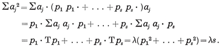
The special case when the a’s are unit vectors was considered long ago by Schlafli,148 who defined such a star by the relation
(a[image]{.image .placeholder original-image-src=“content/images/00114” original-image-title=“” width=“0in” height=“0in”}x)(a[image]{.image .placeholder original-image-src=“content/images/00114” original-image-title=“” width=“0in” height=“0in”}y)=[image]{.image .placeholder original-image-src=“content/images/00114” original-image-title=“” width=“0in” height=“0in”}y, λ=n/s,
for every pair of vectors x, y. (This is clearly equivalent to Tx=λx.) Schläfli showed that the vectors to the vertices of any regular polytope (from its centre) are eutactic ; but he did not think of the eutactic star as forming as a projected cross. That important step was taken by Hadwiger.
[image]
[image]{.image .placeholder original-image-src=“content/images/00114” original-image-title=“” width=“0in” height=“0in”}. A star is eutactic if its symmetry group is irreducible.
[image]{.image .placeholder original-image-src=“content/images/00114” original-image-title=“” width=“0in” height=“0in”}149
[image]{.image .placeholder original-image-src=“content/images/00114” original-image-title=“” width=“0in” height=“0in”}orthogonal shadows of measure polytopes. That conjecture is here, at last, justified.
[]
¶ CHAPTER XIV
STAR-POLYTOPES
[image]
N0 - N1 + N2 - N3 = 0.
[image]
[image]
The density of the star-polytopes takes the strange sequence of values
4, 6, 20, 66, 76, 191.
[image]
[image]{.image .placeholder original-image-src=“content/images/00114” original-image-title=“” width=“0in” height=“0in”} In view of the figures discussed in Chapter VI, it is natural to extend the definition of a polytope so as to allow non-adjacent cells to intersect, and to admit star-polygons and star-polyhedra as elements. Accordingly, we proceed to investigate the possible regular star-polytopes {p, q, r}, where the cell {p, q} and vertex figure {q, r[image]{.image .placeholder original-image-src=“content/images/00114” original-image-title=“” width=“0in” height=“0in”}p, q, r
[image]
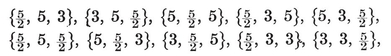
[image]

[image]
Selecting {p, q, r} and {q, r, s[image]{.image .placeholder original-image-src=“content/images/00114” original-image-title=“” width=“0in” height=“0in”}p, q, r, s} :
[image]
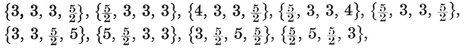
[image]
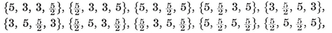
14.15

[image]
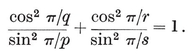
[image]{.image .placeholder original-image-src=“content/images/00114” original-image-title=“” width=“0in” height=“0in”}smaller value of p[image]{.image .placeholder original-image-src=“content/images/00114” original-image-title=“” width=“0in” height=“0in”}greater value of p or s[image]{.image .placeholder original-image-src=“content/images/00114” original-image-title=“” width=“0in” height=“0in”}150 But subtler considerations force us to rule out all[image]
[image]{.image .placeholder original-image-src=“content/images/00114” original-image-title=“” width=“0in” height=“0in”}r
not
The last four sentences afford an instance of the phenomenon of isomorphism151[image]{.image .placeholder original-image-src=“content/images/00114” original-image-title=“” width=“0in” height=“0in”}Fig. 14.2A is a scheme of the twelve “ pentagonal ” polytopes (which all have the same symmetry group [3, 3, 5]), represented as points on a circle. Here, as in Fig. 6.6B[image]
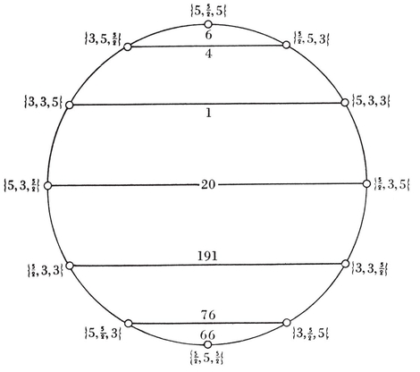
152 it will be seen that the four polytopes
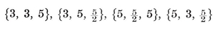
all have the same edges (see Plate IV or VII) ; so also do their four isomorphs

and the pair
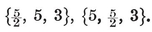
Finally, the following pairs have the same faces :
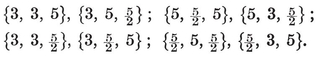
The numbers of elements (see Table I[image]{.image .placeholder original-image-src=“content/images/00114” original-image-title=“” width=“0in” height=“0in”}gp,q,r =14400*, g*3,3 = 24, other gp,q=120, g3
[image]{.image .placeholder original-image-src=“content/images/00114” original-image-title=“” width=“0in” height=“0in”} We proceed to investigate the cases where the vertices of a regular polytope {p, q, r} occur among the vertices of a convex regular polytope, II4[image]{.image .placeholder original-image-src=“content/images/00114” original-image-title=“” width=“0in” height=“0in”}p, q, r[image]
We make use of “ simplified ” sections of II, viz., i0 and i3[image]{.image .placeholder original-image-src=“content/images/00114” original-image-title=“” width=“0in” height=“0in”}0 are distant a from the initial vertex 00, it may happen that they include the vertices of a polyhedron {3, r} of edge a. Then each face of this {3, r} forms with 00 a regular tetrahedron, and such tetrahedra are the cells of a {3, 3, r} inscribed in II. More generally, if the vertices of i0 include the vertices of a {q, r} of edge b, where b/a=2 cos π/p (for some rational value of p), and if a {p, q} of edge a is known to occur in some section of II, then such {p, q}’s are the cells of a {p, q, r} inscribed in II. In fact, the vertex figure of this {p, q, r} is a {q, r} of edge a q, r} inscribed in i0. If i=1 the edges (as well as vertices) of {p, q, r} belong to Π ; in this case the vertex figure of {p, q, r} is obtained by faceting the vertex figure of II.
Since {p, q} must be one of the nine regular polyhedra, the only admissible values for pb/a
If the vertices of the {q, r} of edge b are all the vertices of i0, then we find either a single polytope {p, q, r
d times as many vertices as {p, q, r}. On the other hand, if {q, r} has only some of the vertices of i0, the possibility of a single polytope is ruled out : if i0 includes the vertices of c {q, r}’s, we find a compound
d/c times as many vertices as {p, q, r}. If c and d have a common divisor m (m> 1), it may be possible to pick out d/m of the d {p, q, r}’s so as to form
but such cases will require individual consideration.
Table VIb are those in Table V, multiplied by the values of a in § 6⋅3 (viz., 1, √2, τ, τ√2, τ2) i.e., every b is of the form τu√υ where u=0, 1, 2, 3, 4, or 5, and υ=1, 2, 4, 5, 8 or 10. But b/a must be 1, √2, τ or τ−1. Hence the only sections i0 that concern us are those in which a has the form τu√υ, where u is an integer and υ0 for γ4, where a=√3) are omitted from Table VI. In the case of {5, 3, 3} we also omit sections 20, 40, 100, because they contain no regular polyhedra.
After finding c {q, r}’s of edge b in the section i0, and deducing {p, q} from the relation b/a=2 cos π/p, we can complete the table without difficulty. To fill the column headed “ Location ”, we seek a section that includes one or more {p, q}’s of edge a. If this entry is j0
14⋅31
where e is the number of {p, q}’s in j0d/e times as many cells as {p, q, r}. On the other hand, if the “ location ” of {p, q} is k3
14⋅32
d/e times as many cells as {p, q, r}, e being the number of {p, q}’s in k3), or a compound d{p, q, rd/e times as many cells as {p, q, r}, so that the {p, q}’s inscribed in the k3some of the cells of the d {p, q, r}’s). For instance, in the case of γ4[2β4] (see § 8⋅2), 16 of the 32 cells of the 2 β4’s are inscribed (by pairs) in the 8 cubes of γ4 ; the remaining 16 lie in the bounding hyperplanes of another β4 (reciprocal to the γ4). Again, in the case of
2 [10],
1200 of the 6000 cells of the ten {3, 3, 5}’s are inscribed (by tens) in the 120 dodecahedra of {5, 3, 3} ; the remaining 4800 have a less symmetrical situation.
00 of {3, 3, 5}. This holds also for 14⋅31 and its reciprocal
[d{r, q, p}]′.
Again, whenever two reciprocals are inscribed in reciprocals, their cells occur in “ corresponding ” sections k33 of {3, 3, 5} and {5, 3, 3}, respectively. This holds also for 14⋅32 and its reciprocal
′[d{r, q, p}]′.
These remarks are further illustrations of Pappus’s observation (pages 88 and 238).
We saw, on page 240, that the section 30 of {5, 3, 3} contains an irregular compound of two icosahedra. The symmetry group of this section is, of course, the same as that of 10, namely the extended tetrahedral group. The reflections that occur in this group interchange the two icosahedra ; therefore the rotations are symmetry operations of the separate icosahedra. Hence, if we take one of the ten {3, 3, 5}’s of 2[10], and apply the direct symmetry operations of {5, 3, 3}, we shall obtain the simpler compound
{5, 3, 3}[5],
which uses each vertex of {5, 3, 3} just once. In other words, the ten {3, 3, 5}’s inscribed in {5, 3, 3} fall into two enantiomorphous sets of five (just like the ten tetrahedra inscribed in the dodecahedron). Similarly we find {5, 3, 3}[5
{5, 3, 3}[5{p, q, r}]
where {p, q, r
In view of the existence of the two reciprocal compounds
5[25]{3, 3, 5}, {5, 3, 3}[25]5, it is natural to expect that five of the latter set of twenty-five {3, 4, 3}’s will be inscribed in each {3, 3, 5} of {5, 3, 3}[5],153 giving a simpler (self-reciprocal) compound
14⋅33
This expectation can be justified by referring to § 13⋅6. In fact, the vertices
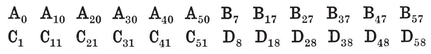
of {3, 3, 5} belong to one inscribed {3, 4, 3}, from which four others may be derived by adding in turn 2, 4, 6, 8 to all the suffix-numbers (i.e., by rotating Fig. 14.3C through successive multiples of 12°).
The reader may be interested to see how the above selection of vertices was made. Fig. 14.3A shows the dodecahedron 20 corresponding to the vertex 00= A0 of {3, 3, 5}. (Its vertices were found by going five steps from A0 along various Petrie polygons.) Fig. 14.3B shows one of the five cubes inscribed in this dodecahedron. This is the section 10 of the desired {3, 4, 3} ; the parallel sections 20 (an octahedron) and 30 (another cube) are shown too. (Each face of the cube 10 is an equatorial square of an octahedron of which 00 is one vertex ; the remaining vertex belongs to 20.) The {3, 4, 3} is then easily completed, as in Fig. 14.3C. By viewing this figure obliquely we can distinguish the sections 13, 23, 33, of Table V (ii).
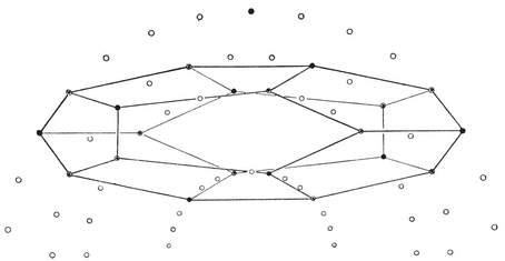
A dodecahedral section of
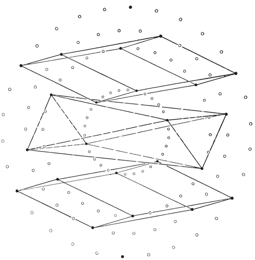
Parallel sections of
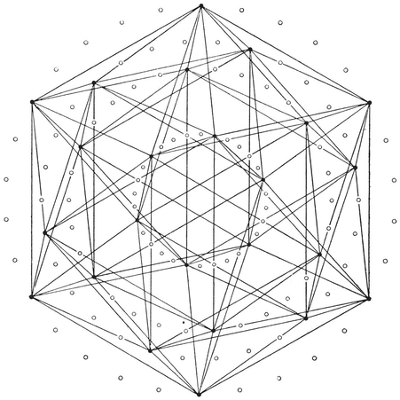
One {3, 4, 3} of {3, 3, 5}[5{3, 4, 3}]
Inscribing β4’s or γ4’s in the {3, 4, 3}’s of 14⋅33, we obtain the two reciprocal compounds
{3, 3, 5}[15 β4]2, 2[15 γ4]{5, 3, 3}.
Collecting results, we see that we have found six self-reciprocal compounds, thirteen reciprocal pairs, and seven compounds which are only vertex-regular. By reciprocating the last seven we obtain seven which are not vertex-regular but “ cell-regular.” (See Table VII on page 305, and Coxeter 18.)
14⋅4. The general regular polytope in four dimensions. The results of §§ 7⋅7 and 7⋅9 remain valid for star-polytopes. In particular, the angles φ=O0 O4 O1 and ψ=O2 O4 O3 are still given by
14⋅41
and
as in 7⋅91. From these we can derive the circum-radius 0R=l csc φ, the other radii jR (as in § 8⋅8), and the dihedral angle π−2ψ. The relation 3R/2R=cos ψ will serve as a check. Alternatively, Table VI (iii) shows that the four polytopes
all have the same circum-radius 0R=2lτ. For the other polytopes inscribed in {3, 3, 5}, the edge 2l is not 1 but a ; so
0R = 2lτ/a.
PLATE VIII
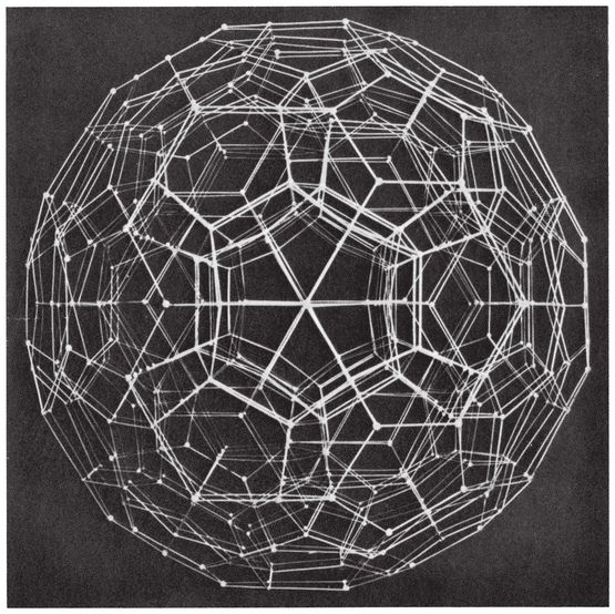
5. 3. 3 }
Defining the volume of {p, q} as in § 6⋅4, we obtain, for the surface-analogue of {p, q, r},
S = N3 Cp,*q*.
With the analogous convention, the content is
Cp, q, r = 3R S/4
(as in 8⋅82). The values in the individual cases can be seen in Table I (on page 295). They may be checked by employing the auxiliary function (j, k) of 8⋅84.
The density d*p*, q, r will be computed in § 14⋅8. We cannot express it by any such simple formula as 6⋅41 or 6⋅42. In fact, the analogue of 6⋅42 is
14⋅42
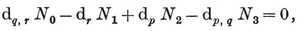
which does not involve d*p*, *q*, r.
To prove 14⋅42, we consider the symmetry group of {p, q, r} and the subgroups which preserve one of the fundamental points O3, O2, O1, O0 (viz., the centre of a cell or face or edge, or a vertex). By 6⋅41, the orders of the subgroups are respectively
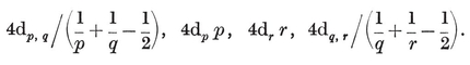
By 7⋅64, these are inversely proportional to the numbers of elements. Hence

[image]
14⋅5. A trigonometrical lemma. In § 6⋅7 we enumerated the possible regular polyhedra with the aid of Gordan’s equation
14⋅51

14⋅52

whose rational solutions may similarly be shown154 to be the permutations of
¶ –
In most applications we shall be led to a slightly different form of this equation, viz.,
14⋅53

whose rational solutions are consequently
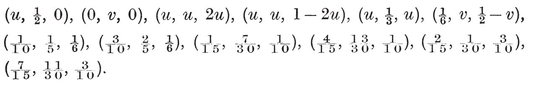
14⋅6. Van Oss’s criterion. In §§ 14⋅2 and 14⋅3 we established the existence of the ten star-polytopes 14⋅11 which, with the six ordinary polytopes 7⋅81, make the grand total sixteen. We now ask why the apparently possible symbols 14⋅12 fail to represent finitely-dense polytopes. The simplest criterion is provided by the remark of van Oss (2, p. 6) that φ must be commensurable with π whenever the vertex figure has central symmetry.
To see this, consider any regular polytope whose vertex figure has central symmetry (e.g., the octahedron, whose vertex figure is a square). The plane joining any edge to the centre O (or O*n) contains a number of edges, forming an “ equatorial ” polygon. Two consecutive sides of this polygon, say AB and BC, contain opposite vertices of the vertex figure at their common vertex B. If the equatorial polygon is a {k}, we have 2φ*=∠AOB=2π/k ; so
14⋅61

Reciprocally, ψ (and the dihedral angle π−2ψ) must be commensurable with π whenever the cell has central symmetry ; for there is then a “ zone ” of cells. Moreover, when both cell and vertex figure have central symmetry, not only ψ and φ but also X will be commensurable with π.
We can begin to construct any one of the would-be polytopes 14⋅12 by fitting cells together in the manner indicated by the Schläfli symbol. The question is, Will the figure eventually close up ? A necessary condition is the closing of the equatorial polygon, and we shall find that this necessary condition is also sufficient.
Van Oss’s criterion would not be of much use in three dimensions ; for it would only apply to {p, q} when {q} has central symmetry, i.e., when the numerator n*q* is even. But it is admirably suitable for the enumeration of polytopes {p, q, r} in four dimensions, since eight of the nine possible vertex figures {q, r} do have central symmetry. In fact, it can be applied in every case except {p, 3, 3}, where there is no question anyhow, as we already know this polytope does exist for p
By 14⋅41 and 14⋅61, every polytope {p, q, r} (where q and r are not both equal to 3) must correspond to a rational solution of the equation
14⋅62
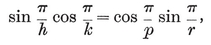
where
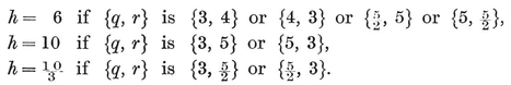
The most obvious solution is k=p, h=r ; but this is irrelevant, as we never have h=r. Another possibility is
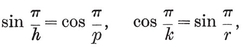
i.e.,
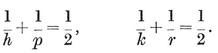
By 2⋅33 (with {p, q} replaced by {q, r}), the numbers p, q, r now satisfy 6⋅71, and we have the nine polytopes
14⋅63
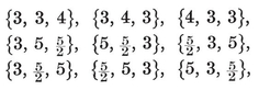
for which k=hp,q. (The occurrence of {4, 3, 3}, with q=r=3, may be regarded as an accident.)
The remaining possibilities (according to 14⋅11 and 14⋅12) are

and the reciprocals of the first and last. Leaving the reciprocals to take care of themselves, we observe that the respective values of h=hq,r are
and that in each case either p=3 or p=r or h=6. Thus 14⋅62 may be replaced by one of the simpler equations
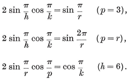
Accordingly, we examine the rational solutions of 14⋅53, to see whether there are any of the form


Thus there are only sixteen regular four-dimensional polytopes : six convex and ten starry. (See Tables I and VIII.)
By examining the distances between pairs of vertices in the notation of § 13·6, we find the following equatorial polygons for the polytopes that have 120 vertices :
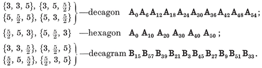
The transition from the decagon to the decagram affords an instance of the following rule for interchanging isomorphic polytopes :
Aj → B7j+15, Bj→D7j−15, Cj→A7j+15, Dj→C7j+15 .
(It is understood that the suffixes are to be reduced modulo 60.)
For the analogous consideration of 14.13, we apply van Oss’s criterion to

whose vertex figures would all have central symmetry. We use 7·72 in the form
sin φ’ cos φ = cos π/p, φ = φp, q, r,s, φ’ = φq, r, s.


Hence there are no regular star*-*polytopes in five or more dimensions.
We shall see, in § 14·9, that there are no regular star-honeycombs either. But van Oss’s criterion is not strong enough to decide that question. The formula naturally gives φ=0 for all 14·14. Incidentally, it makes φ imaginary for all 14·15.
14·7. The Petrie polygon criterion. In four dimensions, van Oss’s criterion amounts to this : if {p, q, r} is a finitely dense polytope, its equatorial polygon must close. Here {p, q} may be any regular polyhedron, and {q, r} any one except {3, 3}. An alternative criterion (cf. page 108), applying without any such exception, is this : if {p, q, r} is a finitely dense polytope, its Petrie polygon must close,1 and ξ2 must be commensurable with π. In other words, if cos π/h1 and cos π/h2 are the positive roots of 12·35, then the Petrie polygon projects into plane polygons {h1} and {h2} in two completely orthogonal planes, so of course the numbers h1 and h2 must be rational.155
From the sum and product of roots of the quadratic equation for X2, we obtain

Hence, for {3, 3, 4} or {4, 3, 3}, h1 h1
h1 h1
h1
The remaining possibilities may be treated by considering the sum and product of cos 2π/h1 and cos 2π/h2 (i.e., of cos ξ1 and cos ξ2), viz.,
For {3, 3, r} we have s=cos 2π*/*r and P=−cos2 π/r ; so
must be a solution of 14·52, and the values of h1 and h2 are as follows :
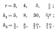


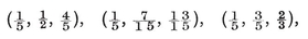
and the corresponding values of cos yπ
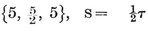
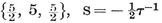
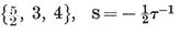 h1 = u1, 2/h2 = 1 − u2, where 2 cos u1π cos u2π = 1 ((0< u1, u2
Comparing this with 14·53, we see that the only rational solution is

 1 =1 − u1, 2/h2 = 1 − u2, where

But the only rational values of (u1, u2
We conclude, as before, that the only regular star-polytopes in four dimensions are 14·11.
The absence of regular star-polytopes in five dimensions may be verified analogously, using the equation

 π
π
It is only fair to point out that the Petrie polygon criterion, like van Oss’s, is inadequate for the discussion of honeycombs.
14·8. Computation of density. Goursat (1, pp. 80-81) proposed a problem analogous to that of Schwarz (§ 6·8): to find all spherical tetrahedra which lead, by repeated reflection in their faces, to a finite set of congruent tetrahedra, i.e., to a honeycomb covering the hypersphere a finite number of times. Clearly, the reflections generate a group, viz. (in the notation of § 11·5),
[m] x [n] or [3, 3] x [1] or [3, 4] x [1] or [3, 5] x [1]
or [3, 3, 3] or [3, 3, 4] or [3, 3, 5] or [3, 4, 3] or [31,1,1].
Hence the faces and their transforms dissect such a tetrahedron into a set of congruent tetrahedra of one of the following shapes :
14·81
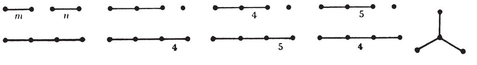
When we compare this with the corresponding statement for Schwarz’s triangles, we are not surprised to find Goursat’s tetrahedra running into hundreds. Their complete enumeration will (perhaps !) be published elsewhere. The essential tool for that formidable work is the following process for deriving them from one another.
If one of Goursat’s tetrahedra has a dihedral angle π/r, where r is fractional, one of the “ virtual mirrors ” will dissect it into two smaller tetrahedra in accordance with the formula
14·82
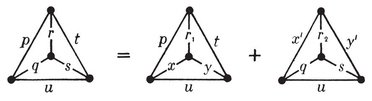
where
(p q r) = (p x r1) + (x’ q r2)
and
(t s r) = ( t y r1) + (y’ s r2).
(See 6·81, and the special cases listed on page 113.) Here, as in § 5·6, each node of the graph denotes a face of the tetrahedron, and a branch marked p indicates the dihedral angle π/p between two faces. Fig. 14.8A shows the dihedral angles at the various edges. The dissecting plane divides the angle π/r into two parts, π/r1 and π/r2, and cuts the opposite edge at X. On spheres drawn round the four vertices of the whole tetrahedron, the trihedra cut out Schwarz’s triangles
(p q r), (t s r), (p t u), (q s u).
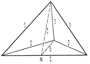
Dissecting a tetrahedron
The first two of these are dissected into (p x r1) + (x′ q r2) and (t y r1) + (y’ s r2). But the other two, viz.,

and

are retained in the respective parts. (See 14·82.) In practice many of the dihedral angles are right angles, and then we omit the corresponding branches of the graph. As before, an unmarked branch will stand for a branch marked “3” (meaning “angle π/3 ”).
Our present purpose is to obtain an alternative proof for the existence of the ten star-polytopes 14·11 (independent of the rather tiresome details of §§ 14·2 and 14·3), and to compute their densities.
Let O4 be the centre of one of these polytopes, O3 the centre of a cell, O2 the centre of a face of that cell, O1 the mid-point of a side of that face, O0 the vertex at one end of that side. We can project the tetrahedron O0 O1 O2 O3 from O4 into a spherical tetrahedron P0 P1 P2 P3. Conversely, beginning with the spherical tetrahedron, we can reconstruct the polytope by combining the reflections in the tetrahedron’s faces and considering all the transforms of P0. Thus P0 P1 P2 P3 is a quadrirectangular tetrahedron (or orthoscheme), and
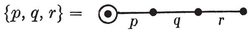
(cf. 11·71). Accordingly, we are interested in the special tetrahedra
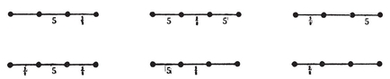
which appear (as D, F, J, O, P, R) in the following list of seventeen particular cases of the dissection 14·82 :
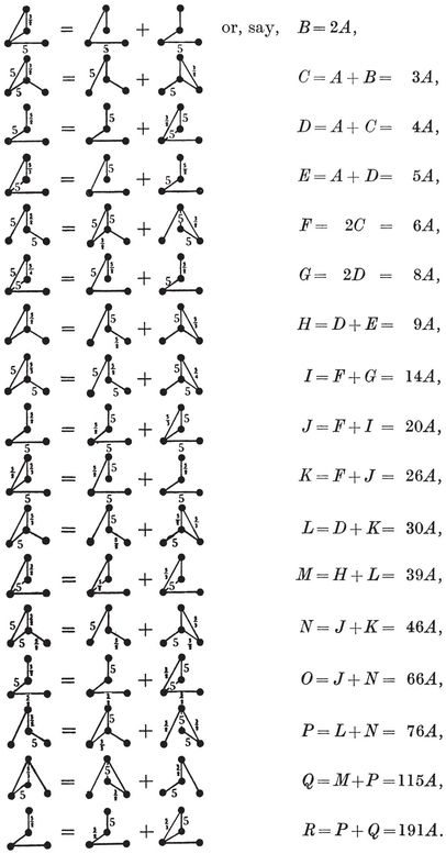
From this list we extract the significant items
D = 4A, F = 6A, J = 20A, O = 66A, P = 76A, R = 191A,
which reveal the densities of the regular star-polytopes, as recorded in Fig. 14.2A. In fact, since the 14400 characteristic tetrahedra of {3, 3, 5} fill the spherical space just once, the equation
R = 191A,

14·9. Complete enumeration of regular star-polytopes and honeycombs. A similar method may be used for excluding 14·12 (without appealing to § 14·5, which is so difficult to prove). We dissect the corresponding tetrahedra as follows :
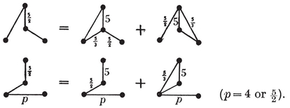

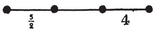 π/5 and π
Similarly, to exclude 14·13, we consider the spherical simplexes

where p=3,
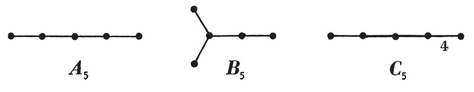
(see Table IV). Hence 14·13 must all be ruled out as having infinite density, and we see again that there are no regular star-polytopes in five or more dimensions. Star-honeycombs would have such polytopes for cells or vertex figures ; hence there are no regular star-honeycombs in five or more dimensions.
The same kind of argument settles the question of the existence of star-honeycombs in four dimensions. Simplicial subdivision of the apparently possible honeycombs 14·14 would lead to Euclidean simplexes, of which the first is the Y5 of § 11·4, while the Euclidean nature of the others may be checked similarly, as follows :

Obviously none of these simplexes can be built up from repetitions of any of
Hence 14·14 must all be excluded as having infinite density : there are no regular star-honeycombs at all.
14·x. Historical remarks. π/3. We may justify his stopping there by remarking that, from the standpoint of topology, the six figures which he missed are not manifolds but only pseudo-manifolds.
Edmund Hess was born in 1843, took his doctorate at Marburg in 1866 (with a dissertation on the flow of air through a small orifice), wrote a number of papers on polytopes, edited Hessel 1 for Ostwald’s Klassiker p, q, r}, we may be sure that he was not aware of Schläfli’s work. But he computed all the densities, understood the relation between reciprocals, and obtained the formula 14·42.
 φ
φ π. (van Oss 2, p. 6.) Our § 14·5 is designed to remedy that deficiency. (The above theorem of Hess is thus finally established.) § 14·7 provides a full account of the alternative criterion outlined in Coxeter 3, p. 203.
We saw, in 13·61, that {3, 3, 5} has Petrie polygons
A0 A2 A4 . . . A58 and D0 D22 D44 . . . D38,
Tafel VIII. By taking alternate vertices we obtain the skew 15-gons
A0 A4 A8 . . . A56 and D0 D16 D32 … D44,
 Tafel VIa
 Tafel VIIa
In § 14·8 we computed the volumes of the various characteristic tetrahedra by the strictly elementary process of dissection. It is interesting to recall that Schläfli (4, pp. 101-102, formulae (4)-(6), (8)-(11)) computed these same volumes in terms of his function f(π/p, π/q, π/r), which enables us to express the density of each star-polytope in the form
Of the forty-six compounds that arose as by-products in § 14·3, eleven were discovered by Schoute (6, pp. 215, 216, 231 ; cf. Coxeter 4, p. 337). The rest are new, except
{5, 3, 3} [120 α4] {3, 3, 5},
which is due to Urech (1, p. 47) and was almost anticipated by Hess (4, p. 48) in his observation that [3, 3, 5] has a subgroup [3, 3, 3].
To save space, we have disregarded the possibility of compounds in more than four dimensions. Actually, there are none in five or six dimensions. In seven and eight we find
cγ*7[16cα7]cβ7,* cγ8[16cβ8], [16cγ8]cβ8,
where c = 1, 15 or 30. The case c = 1 can be generalized to
γn−1[dαn−1]βn−1, γn[dβn], [dγn]βn,
where n=2*k* k=2, 3, 4, … ). The theory of these compounds is connected with orthogonal156 matrices of ± 1’s. (For proofs of such statements, see Schoute 5, Barrau 1157 and Coxeter 4.) Similarly, the theory of compound honeycombs
δ*n[dδn]δn*.
is connected with orthogonal156 matrices of integers.
[]
¶ EPILOGUE
WE have now reached the end of our journey. On the way, we visited most of the domains of elementary mathematics (and some not so elementary) : algebra, synthetic and analytic geometry, plane and spherical trigonometry, integral calculus (in § 7·3), the kinematics of a rigid body, the theory of groups, and topology.
We began with the five Platonic solids, obtaining their numerical and metrical properties in Chapters I and II, their symmetry groups in Chapters III and V. We saw that they fall naturally into two classes : (i) the “ crystallographic ” solids α3 (the tetrahedron), β3 (the octahedron), and γ3 (the cube) ; (ii) the icosahedron and dodecahedron, which form, with the four Kepler-Poinsot solids, a set of six “ pentagonal ” polyhedra (Fig. 6.6B), all having the same symmetry group. We found that the crystallographic solids have n-dimensional analogues, whose properties are just such as would be inferred by pure analogy. On the other hand, the pentagonal polyhedra are related to twelve pentagonal polytopes in four dimensions (Fig. 14.2A), and there the family comes to an abrupt end. Another peculiarity of four-dimensional space is the occurrence of the 24-cell {3, 4, 3}, which stands quite alone, having no analogue above or below.
For a strict discussion of regular polytopes, this would be the whole story. But it seemed worth while (in Chapter XI) to show how the simplexes and cross polytopes occur, qua ki0 and k11, as members of an interesting family of “uniform” polytopes kij in n dimensions, where
n = i + j + k + 1 > ijk − 1.
Here the significant number of dimensions is not four but eight.
A more detailed summary of our results can best be given in the form of tables. These are preceded by some definitions of the tabulated properties.
[]
¶ DEFINITIONS OF SYMBOLS USED IN THE FOLLOWING TABLES
Table I (i). Each polyhedron {p, q} has N0 vertices, N1 edges, N2 faces {p}, and vertex figure {q}. Its complete symmetry group [p, q] is of order g = 4N1. The Petrie polygon projects into an {h} in a suitable plane. The density is d. The characteristic (spherical) triangle has sides φ, χ, ψ (opposite to angles π/p, π/2, π/q). These are conveniently expressed in terms of the special angles

The dihedral angle is π − 2ψ. Taking the edge-length to be 2l, the radii are 0R, 1R, 2R, the surface is S, and the volume is C. These properties are connected by such formulae as 1·71 and 5·43 (when d= 1), 2·21, 2·33, 2·42-2·46, 6·41-6·43.
Table I (ii). Each polytope {p, q, r} has N0 vertices, N1 edges, N2 faces {p}, N3 cells {p, q}, and vertex figure {q, r}. Its symmetry group [p, q, r] is of order g. The equatorial polygon (except when q=r=3), is a {k}. The Petrie polygon, a skew h-gon, projects into an {h1} in one plane and an {h2} in the completely orthogonal plane. Three dihedral angles of the characteristic tetrahedron (Fig. 7.9A) are right angles ; the other three are π/p, π/q, π/r, and occur at edges of lengths ψ, χ, φ. These are conveniently expressed in terms of the special angle
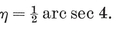
The circum- and in-radii are 0R and 3R, the sum of the volumes of the cells is S, and the four-dimensional content or hyper-volume is C. These properties are connected by such formulae as 7·64, 7·65, 7·71, 7·91, 8·82 and 8·86 (with *n=*4), 12·35 (which has roots cos π/h1, cos π/h2), and 14·61.
Table I (iii). The polytopes αn, βn, γn occur for every positive integer n; when n ≥ 5 they stand alone. Their properties, analogous to those defined above, are connected by such formulae as 7·62, 7·63, 8·81, 8·82, 8·87, and 12·33 (which has roots cos π/hk).
Table II. The regular honeycombs fill n-dimensional Euclidean space homogeneously, in the sense that the numbers of j-dimensional elements in a large portion tend to be proportional to definite numbers vj (which are inversely proportional to gp, . . . , r gu, . . . , w, in the notation of 7·63).
Table III. (p q r) means a spherical triangle with angles π/p, π/q, π/r
Table IV. In the graphical symbols, nodes represent walls or mirrors, perpendicular whenever the nodes are not directly joined by a branch, but otherwise inclined at an internal angle π/3 or π/k according as the branch is unmarked or marked k. An stands for a simple chain of n nodes (and n−1 unmarked branches), Pn+1 for an (n+1)-gon, and so on. For each spherical simplex we have given the order of the corresponding group, as computed in 7·66, 7·67, 8·22, 8·51, 11·74, 11·81-11·83.
Table V (i), (iii), (v). For a regular polytope of edge 2l, each section includes all vertices distant 2la from a given vertex. Among these vertices we seek regular polyhedra of edge 2lb, for use in Table VI, as follows.
Table VI. Such a regular polyhedron {q, r}, of edge b (taking 2l=1), is the vertex figure of a polytope {p, q, r}, whose cell {p, q} occurs in the section listed under “ Location ”.
Table VII. Here c{l, m, n}[d{p, q, r}]e{s, t, u} means a compound of d {p, q, r}’s having the vertices of an {l, m, n}, each taken c times, and the bounding hyperplanes of an {s, t, u}, each taken e times.
TABLE I :
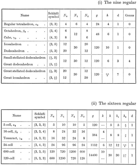
REGULAR POLYTOPES
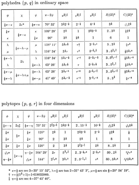
TABLE I: REGULAR
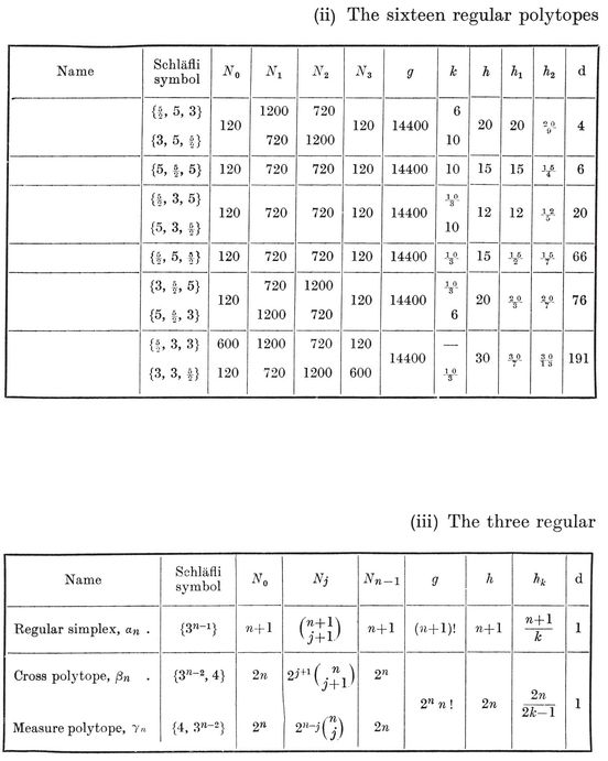
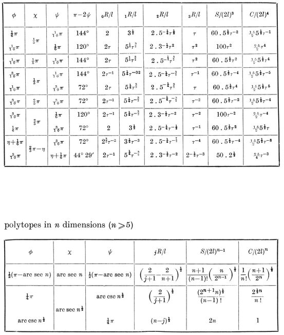
TABLE II : REGULAR HONEYCOMBS
(§§ 4·1, 4·8, 7·2, 8·5, 9·8)
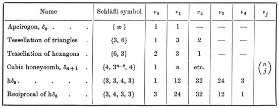
TABLE III : SCHWARZ’S TRIANGLES
(§ 6·8)
¶ –
TABLE IV: FUNDAMENTAL REGIONS FOR IRREDUCIBLE GROUPS GENERATED BY REFLECTIONS
[image]
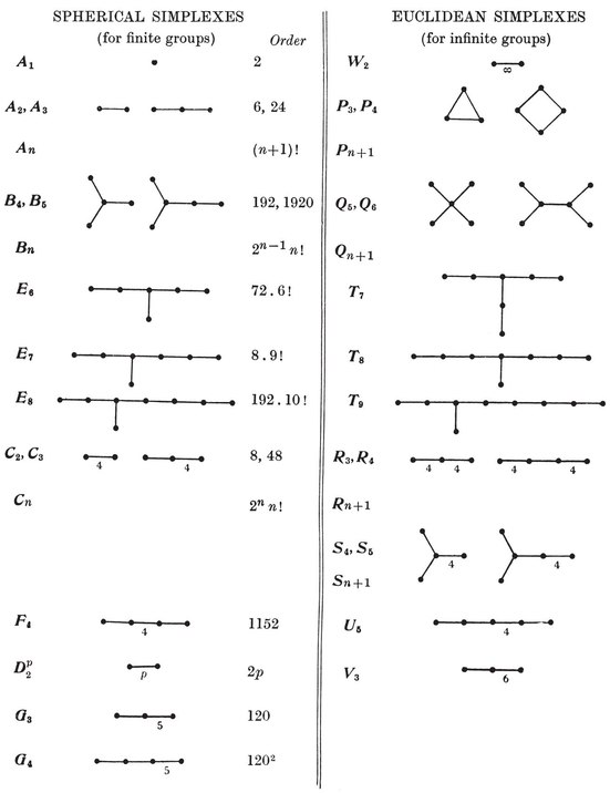
TABLE V[image]
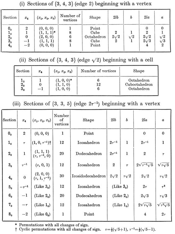
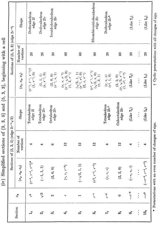
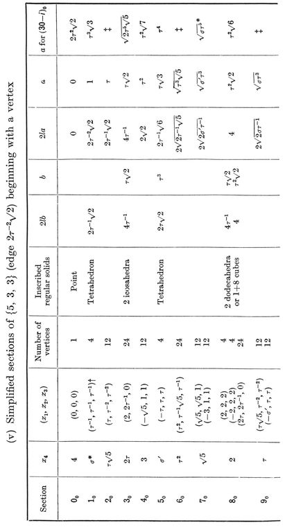
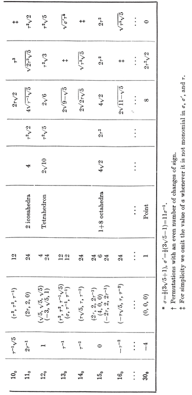
THE DERIVATION OF FOUR-DIMENSIONAL STAR-POLYTOPES AND COMPOUNDS BY FACETING THE CONVEX REGULAR POLYTOPES II
[image]
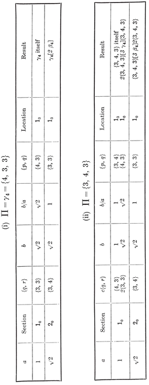
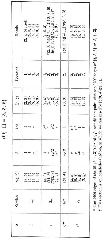
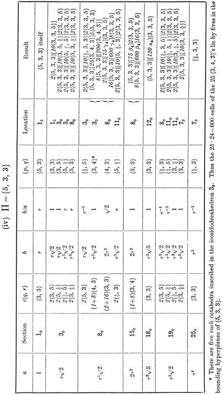
REGULAR COMPOUNDS IN FOUR DIMENSIONS
[image]
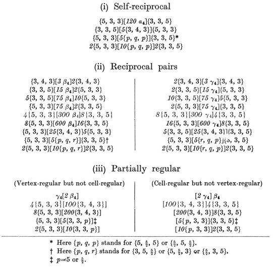
THE NUMBER OF REGULAR POLYTOPES AND HONEYCOMBS IN n DIMENSIONS (INCLUDING STAR-POLYTOPES BUT NOT COMPOUNDS)
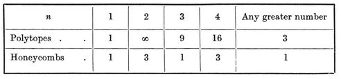
[]
¶ BIBLIOGRAPHY
Abbott 1. Flatland: a romance of many dimensions, by A Square. Boston, 1885 and 1928. (Dover Reprint)
Andreini 1. Sulle reti di poliedri regolari e semiregolari. Memorie della a Società italiana delle Scienze (3), 14 (1905), pp. 75-129.
Badoureau 1. Mémoire sur les figures isoscèles. Journal de l’École Polytechnique, 49 (1881), pp. 47-172.
Baker 1. Principles of Geometry. Vol. IV. Cambridge, 1925.
Ball 1. Mathematical Recreations and Essays (11th edition). London, 1959.
Barrau 1. Die zentrische Zerlegung der regulären Polytope. Nieuw Archief voor Wiskunde (2), 7 (1906), pp. 250-270.
Bentley and Humphreys 1. Snow Crystals. New York, 1931. (Dover)
Bilinski 1. Über die Rhombenisoeder. Glasnik, 15 (1960), pp. 251-263.
Birkhoff and MacLane 1. A Survey of Modern Algebra. New York, 1941.
Brahana 1. Regular maps and their groups. American Journal of Mathematics, 49 (1927), pp. 268-284.
Brauer and Coxeter 1. A generalization of theorems of Schönhardt and Mehmke on polytopes. Transactions of the Royal Society of Canada, 34 (1940), Section III, pp. 29-34.
Bravais 1. Mémoire sur les polyèdres de forme symétrique. Journal de Mathématiques (1), 14 (1849), pp. 141-180.
Brückner 1. Vielecke und Vielflache. Leipzig, 1900.
———2. Über die gleicheckig-gleich flächigen, diskontinuierlichen und nichtkonvexen Polyeder. Abhandlungen (= Nova Acta) der Kaiserlichen Leopoldinisch-Carolinischen Deutschen Akademie der Naturforscher, 86 (1906), pp. 1-348.
Burckhardt 1. Über konvexe Körper mit Mittelpunkt. Vierteljahrsschrift der Naturforschenden Gesellschaft in Zürich, 85 (1940), pp. 149-154.
———2. Die Bewegungsgruppen der Kristallographie. Basel, 1947. Burnside 1. On a configuration of twenty-seven hyper-planes in four-dimensional space. Proceedings of the Cambridge Philosophical Society, 15 (1910), pp. 71-75.
———2. The determination of all groups of rational linear substitutions of finite order which contain the symmetric group in the variables. Proceedings of the London Mathematical Society (2), 10 (1912), pp. 284-308.
Caravelli 1. Traité des hosoèdres. Paris, 1959.
Cartan 1. La géométrie des groupes simples. Annali di Matematica (4), 4 (1927), pp. 209-256.
———2. Complément au mémoire sur la géometrie des groupes simples. Ibid., 5 (1928), pp. 253-260. 306
Catalan 1. Mémoire sur la théorie des polyèdres. Journal de 1 École Polytechnique, 41 (1865), pp. 1-71.
Cauchy 1. Recherches sur les polyèdres. Journal de l’École Polytechnique, 16 (1813), pp. 68-86.
Cayley 1. On the theory of groups, as depending on the symbolic equation θn = 1. Philosophical Magazine (4), 7 (1854), pp. 40-47 ; or Collected Mathematical Papers, 2 (1889), pp. 123-130.
———2. On Poinsot’s four new Regular Solids. Philosophical Magazine (4), 17 (1859), pp. 123-128; or Collected Mathematical Papers, 4 (1891), pp. 81-85.
Cesàro 1. Forme poliedriche regolari e semi-regolari in tutti gli spazii.[image]
Courant 1. Vorlesungen über Differential- und Integralrechnung. Vol. 2. Berlin, 1931. Translated by E. J. McShane as Differential and Integral Calculus (Vol. 2), New York, 1936.
Coxeter 1. The pure Archimedean polytopes in six and seven dimensions. Proceedings of the Cambridge Philosophical Society, 24 (1928), pp. 1-9.
———2. Groups whose fundamental regions are simplexes. Journal of the London Mathematical Society, 6 (1931), pp. 132-136.
———3. The densities of the regular polytopes. Proceedings of the Cambridge Philosophical Society, 27 (1931), pp. 201-211 ; 28 (1932), pp. 509-531.
———4. Regular compound polytopes in more than four dimensions. Journal of Mathematics and Physics, 12 (1933), pp. 334-345.
———5. Discrete groups generated by reflections. Annals of Mathematics, 35 (1934), pp. 588-621.
———6. The functions of Schläfli and Lobatschefsky. Quarterly Journal of Mathematics, 6 (1935), pp. 13-29.
———7. Wythoff’s construction for uniform polytopes. Proceedings of the London Mathematical Society (2), 38 (1935), pp. 327-339.
———8. On Schläfli’s generalization of Napier’s Pentagramma Mirificum. Bulletin of the Calcutta Mathematical Society, 28 (1936), pp. 123-144.
———9. Regular skew polyhedra in three and four dimensions. Proceedings of the London Mathematical Society (2), 43 (1937), pp. 33-62.
———10. An easy method for constructing polyhedral group-pictures. American Mathematical Monthly, 45 (1938), pp. 522-525.
———11. Lösung der Aufgabe 245. Jahresbericht der Deutschen Mathematiker-Vereinigung, 49 (1939), pp. 4-6.
———12. The groups Gm, n, p. Transactions of the American Mathematical Society, 45 (1939), pp. 73-150.
———13. Regular and semi-regular polytopes. Mathematische Zeitschrift, 46 (1940), pp. 380-407.
Coxeter 14. The polytope 221, whose 27 vertices correspond to the lines on the general cubic surface. American Journal of Mathematics, 62 (1940), pp. 457-486.
———15. The map-coloring of unorientable surfaces. Duke Mathematical Journal, 10 (1943), pp. 293-304.
———16. Integral Cayley numbers. Duke Mathematical Journal, 13 (1946), pp. 561-578.
———17. The nine regular solids. Proceedings of the First Canadian Mathematical Congress (Toronto, 1946), pp. 252-264.
———18. Regular honeycombs in elliptic space. Proceedings of the London Mathematical Society (3), 4 (1954), pp. 471-501.
———19. Twelve Geometric Essays. Carbondale, Illinois, 1968.
———20. Introduction to Geometry. New York, 1961.
———21. Regular Complex Polytopes. Cambridge, England, 1973.
Coxeter, Du Val, Flather, and Petrie 1. The Fifty-nine Icosahedra. University of Toronto Studies (Mathematical Series), 6 (1938), pp. 1-26.
Curjel 1. Notes on the regular hypersolids. Messenger of Mathematics, 28 (1899), pp. 190-191.
Dickson 1. Algebras and their Arithmetics. Chicago, 1923. (Dover)
Donnay 1. Derivation of the Thirty-two Point-Groups. University of Toronto Studies (Geological Series), 47 (1942), pp. 33-51.
Dürer 1. Underweysung der messung mit dem zirckel und richtscheyt in linien, ebnen unnd gantzen corporen. Nürnberg, 1525.
Du Val 1. On the directrices of a set of points in a plane. Proceedings of the London Mathematical Society (2), 35 (1933), pp. 23-74.
———2. On isolated singularities of surfaces which do not affect the conditions of adjunction. Proceedings of the Cambridge Philosophical Society, 30 (1934), pp. 453-465, 483-491.
———3. The unloading problem for plane curves. Americal Journal of Mathematics, 62 (1940), pp. 307-311.
Dyck 1. Gruppentheoretische Studien. Mathematische Annalen, 20 (1882), pp. 1-44.
Elte 1. The Semiregular Polytopes of the Hyperspaces. Groningen, 1912.
Euler 1. Elementa doctrinae solidorum. Novi commentarii Academiae scientiarum imperialis petropolitanae ( = Akademiya nauk Leningrad), 4 (1752), pp. 109-160.
Ewald 1. Das “ reziproke Gitter ” in der Strukturtheorie. Zeitschrift fur Krystallographie, 56 (1921), pp. 129-156.
Fedorov 1. Elemente der Gestaltenlehre. Mineralogicheskoe obshchestvo, Leningrad ( = Verhandlungen der Russisch-Kaiserlichen Mineralo-gischen Gesellschaft zu St. Petersburg) (2), 21 (1885), pp. 1-279 (especially pp. 193-198). Abstract in Zeitschrift für Krystallographie und Mineralogie, 21 (1893), pp. 688-689.
Fedorov 2. The numerical relation between the zones and faces of a polyhedron. Mineralogical Magazine, 18 (1919), pp. 99-100.
Forchhammer 1. Prφver paa Geometri med fire Dimensioner. Tidsskrift for Mathematik (4), 5 (1881), pp. 157-166.
Ford 1. Automorphic Functions. New York, 1929.
Franklin 1. Hypersolid concepts, and the completeness of things and phenomena. Mathematical Gazette, 21 (1937), pp. 360-364.
Gergonne 1. Recherches sur les polyèdres, renfermant en particulier un commencement de solution du problème proposé à la page 256 du septième volume des Annales. Annales de Mathématiques pures et appliquées, 9 (1819), p. 321.
Gordan 1. Ueber endliche Gruppen linearer Transformationen einer Veränderlichen. Mathematische Annalen, 12 (1877), pp. 23-46.
Gosset 1. On the regular and semi-regular figures in space of n dimensions. Messenger of Mathematics, 29 (1900), pp. 43-48.
Goursat 1. Sur les substitutions orthogonales et les divisions régulières de l‘espace. Annales Scientifiques de l’École Normale Supérieure (3), 6 (1889), pp. 9-102.
Hadwiger 1. Über ausgezeichnete Vektorsterne und reguläre Polytope. Commentarii Mathematici Helvetici, 13 (1940), pp. 90-107.
Hamilton 1. Memorandum respecting a new System of Roots of Unity. Philosophical Magazine (4), 12 (1856), p. 446.
Haussner 1. Abhandlungen über die regelmässigen Sternkörper, von L. Poinsot (1809), A. L. Cauchy (1811), J. Bertrand (1858), A. Cayley (1859). Leipzig, 1906.
Heath 1, 2. A History of Greek Mathematics. (Two volumes.) Oxford, 1921.
Herschel 1. Sir Wm. Hamilton’s Icosian Game. Quarterly Journal of pure and applied Mathematics, 5 (1862), p. 305.
Hess 1. Ueber die zugleich gleicheckigen und gleichflächigen Polyeder.[image]
———2. Über vier Archimedeische Polyeder höherer Art. Kassel, 1878.
———3. Einleitung in die Lehre von der Kugelteilung. Leipzig, 1883.
———4. Über die regulären Polytope höherer Art. Sitzungsberichte der Gesellschaft zur Beförderung der gesammten Naturwissenschaften zu Marburg, 1885, pp. 31-57.
———5. Über die Zahl und Lage der Bilder eines Punktes bei drei eine Ecke bildenden Planspiegeln. Ibid., 1888.
Hessel 1. Krystallometrie, oder Krystallonomie und Krystallographie. (Ostwald’s Klassiker der exakten Wissenschaften, 88 and 89.) Leipzig, 1897.
———2. Uebersicht der gleicheckigen Polyeder. Marburg, 1871.
Hessenberg 1. Vektorielle Bergründung der Differentialgeometrie. Mathematische Annalen, 78 (1917), pp. 187-217.
Hilton 1. Note on the thirty-two classes of symmetry. Mineralogical Magazine, 14 (1906), pp. 261-263.
Hinton 1. A New Era of Thought. London, 1888.
Hirsch 1. Sammlung geometrischer Aufgaben. Vol. 2. Berlin, 1807.
Hoppe 1. Regelmässige linear begrenzte Figuren von vier Dimensionen. Archiv der Mathematik und Physik, 67 (1882), pp. 29-43.
———2. Berechnung einiger vierdehnigen Winkel. Ibid., 67 (1882), pp. 269-290.
———3. Die regelmässigen linear begrenzten Figuren jeder Anzahl von Dimensionen. Ibid., 68 (1882), pp. 151-165.
Infeld 1. Whom the Gods Love. New York, 1948.
Jouffret 1. Traité élémentaire de géométrie à quatre dimensions. Paris, 1903.
Kelvin and Tait 1. Nautral Philosophy. Cambridge, 1888.
Kepler 1. Harmonice Mundi. Opera Omnia : Vol. 5. Frankfurt, 1864.
Klein 1. Vorlesungen über das Ikosaeder und die Auflösung der Gleichungen fünften Grades. Leipzig, 1884. Translated by G. G. Morris as Lectures on the Icosahedron, London, 1913.
———2. Elementarmathematik vom höheren Standpunkte aus. Vol. 1. Berlin, 1924. Translated by E. R. Hedrick and C. A. Noble as Elementary Mathematics from an Advanced Standpoint, New York, 1932.
König 1. Theorie der endlichen und unendlichen Graphen. Leipzig, 1936.
Kowalewski 1. Der Keplersche Körper und andere Bauspiele. Leipzig, 1938.
Levi 1. Algebra. Vol. 1. Calcutta, 1942.
Lucas 1. Récréations Mathématiques. Vol. 2. Paris, 1883.
———2. Théorie des Nombres. Vol. 1. Paris, 1891.
Lyche 1. Un théorème sur les determinants. Det Kongelige Norske Videnskabers Selskab Forhandlinger, 1 (1928), pp. 119-120.
Manning 1. Geometry of Four Dimensions. New York, 1914. (Dover)
Meier Hirsch. See Hirsch.
Miller 1. A Treatise on Crystallography. Cambridge, 1839.
Minkowski 1. Zur Theorie der Einheiten in den algebraischen Zahlkörpern. Nachrichten von der Königlichen Gesellschaft der Wissenschaften und der Georg-Augusts-Universität zu Göttingen, 1900, pp. 90-93; or Gesammelte Abhandlungen, 1 (1911), pp. 316-319.
Möbius 1. Ueber das Gesetz der Symmetrie der Krystalle und die Anwendung dieses Gesetzes auf die Eintheilung der Krystalle in Systeme. Journal fur die reine und angewandte Mathematik, 43 (1852), pp. 365-374 ; or Gesammelte Werke, 2 (1886), pp. 349-360.
———2. Zur Theorie der Polyëder und der Elementarverwandtschaft. Gesammelte Werke, 2 (1886), pp. 515-559.
———3. Theorie der symmetrischen Figuren. Ibid., pp. 561-708.
Moore 1. Concerning the abstract groups of order k! andholohedrically isomorphic with the symmetric and the alternating substitution-groups on k letters. Proceedings of the London Mathematical Society (1), 28 (1897), pp. 357-366.
Neville 1. The Fourth Dimension. Cambridge, 1921.
Niggli 1. Die Flächensymmetrien homogener Diskontinuen. Zeitschrift für Krystallographie und Mineralogie, 60 (1924), pp. 283-298.
van Oss 1. Das regelmässige Sechshundertzell und seine selbstdeckenden Bewegungen.[image]
———2. Die regelmässigen vierdimensionalen Polytope höherer Art.[image]
Pascal 1. Die Determinanten. Leipzig, 1900.
Pitsch 1. Über halbreguläre Sternpolyeder. Zeitschrift für das Real-schulwesen, 6 (1881), pp. 9-24, 64-65, 72-89, 216.
Poincaré 1. Sur la généralisation d‘un théorème d’Euler relatif aux polyèdres. Comptes rendus hebdomadaires des séances de l’Académie des Sciences, Paris, 117 (1893), pp. 144-145.
———2. Complément a l’Analysis Situs. Rendiconti del Circolo Matematico di Palermo, 13 (1899), pp. 285-343.
Poinsot 1. Mémoire sur les polygones et les polyèdres. Journal de l’École Polytechnique, 10 (1810), pp. 16-48.
Pólya 1. Über die Analogie der Kristallsymmetrie in der Ebene. Zeitschrift für Krystallographie und Mineralogie, 60 (1924), pp. 278-282.
Puchta 1. Analytische Bestimmung der regelmässigen convexen Körper im Raum von vier Dimensionen nebst einem allgemeinen Satz aus des Substitutionstheorie.[image]
Richmond 1. The volume of a tetrahedron in elliptic space. Quarterly Journal of pure and applied Mathematics, 34 (1903), pp. 175-177.
Riemann 1. Theorie der Abel’schen Functionen. Journal fur die reine und angewandte Mathematik, 54 (1857), pp. 115-155 ; or Gesammelte Mathematische Werke (1892), pp. 88-144.
Robinson 1. On the fundamental region of a group, and the family of configurations which arise therefrom. Journal of the London Mathematical Society, 6 (1931), pp. 70-75.
———2. On the orthogonal groups in four dimensions. Proceedings of the Cambridge Philosophical Society, 27 (1931), pp. 37-48.
Rohrbach 1. Bemerkungen zu einem Determinantensatz von Minkowski. Jahresbericht der Deutschen Mathematiker-Vereinigung, 40 (1931), pp. 49-53.
Room 1. The Schur quadrics of a cubic surface (I). Journal of the London Mathematical Society, 7 (1932), pp. 147-164.
*Rudel **1.***Vom Körper höherer Dimension. Kaiserlautern, 1882.
Schläfli 1. Réduction d‘une Intégrale Multiple qui comprend l’arc du cercle et l’aire du triangle sphérique comme cas particuliers. Journal de Mathématiques (1), 20 (1855), pp. 359-394.
——— 2. An attempt to determine the twenty-seven lines upon a surface of the third order, and to divide such surfaces into species in reference to the reality of the lines upon the surface. Quarterly Journal of pure and applied Mathematics, 2 (1858), pp. 110-120.
——— 3. On the multiple integral ∫n dx dy … dz, whose limits are p1 = a1x + b1y + … + h1z > 0, p2 > 0, . . . , pn > 0 ; and x2 + y2 + … + z2 < 1. Quarterly Journal of pure and applied Mathematics, 2 (1858), pp. 269-301; 3 (1860), pp. 54-68, 97-108.
———4. Theorie der vielfachen Kontinuität. Denkschriften der Schweizerischen naturforschenden Gesellschaft, 38 (1901), pp. 1-237.
Schlegel 1. Theorie der homogen zusammengesetzten Raumgebilde. Verhandlungen (= Nova Acta) der Kaiserlichen Leopoldinisch-Carolinischen Deutschen Akademie der Naturforscher, 44 (1883), pp. 343-459.
———2. Ueber Projektionsmodelle der regelmässigen vierdimensionalen Körper. Waren, 1886.
Schönemann 1. Über die Konstruktion und Darstellung des Ikosaeders und Sterndodekaeders. Zeitschrift fur Mathematik und Physik von Schlömilch-Cantor, 18 (1873), pp. 387-392.
Schoute 1. Le déplacement le plus général dans l‘espace à n dimensions. Annales de l’École Polytechnique de Delft, 7 (1891), pp. 139-158.
———2. Regelmässige Schnitte und Projektionen des Hundertzwanzigzelles und Sechshundertzelles im vierdimensionalen Raume[image]
———3. Het vierdimensionale prismoïde.[image]
———4. Mehrdimensionale Geometrie. Vol. 1 (Die linearen Räume). Leipzig, 1902.
———5. Centric decomposition of polytopes. Koninklijke Akademie van Wetenschappen te Amsterdam, Proceedings of the Section of Sciences, 6 (1904), pp. 366-368.
———6. Mehrdimensionale Geometrie. Vol. 2 (Die Polytope). Leipzig, 1905.
———7. Regelmässige Schnitte und Projektionen des Hundertzwanzigzelles und Sechshundertzelles im vierdimensionalen Raume[image]
———8. The sections of the net of measure polytopes M*n* of space Sp*n* with a space Sp*n*−1 normal to a diagonal. Koninklijke Akademie van Wetenschappen te Amsterdam, Proceedings of the Section of Sciences, 10 (1908), pp. 688-698.
Schoute 9. On the relation between the vertices of a definite six-dimensional polytope and the lines of a cubic surface. Ibid., 13 (1910), pp. 375-383.
——10. Analytical treatment of the polytopes regularly derived from the regular polytopes[image]
Schwarz 1. Elementarer Beweis des Pohlke’schen Fundamentalsatzes der Axonometrie. Journal fur die reine und angewandte Mathematik, 63 (1864), pp. 309-314 ; or Gesammelte Mathematische Abhandlungen, 2 (1890), pp. 1-7.
——2. Zur Theorie der hypergeometrischen Reihe. Ibid., 75 (1873), pp. 292-335 ; or Gesammelte Mathematische Abhandlungen, 2, pp. 211-259.
Sommerville 1. Division of space by congruent triangles and tetrahedra. Proceedings of the Royal Society of Edinburgh, 43 (1923), pp. 85-116.
——2. The regular divisions of space of n dimensions and their metrical constants. Rendiconti del Circolo Matematico di Palermo, 48 (1924), pp. 9-22.
——3. An Introduction to the Geometry of n Dimensions. London, 1929.
Speiser 1. Die Theorie der Gruppen von endlicher Ordnung. Berlin, 1937.
von Staudt 1. Geometric der Lage. Nürnberg, 1847.
Steinberg 1. On the number of sides of a Petrie polygon. Canadian Journal of Mathematics, 10 (1958), pp. 220-221.
——2. Finite reflection groups. Transactions of the American Mathematical Society, 91 (1959), pp. 493-504.
Steinhaus 1. Mathematical Snapshots. New York, 1938.
Steinitz und Rademacher 1. Vorlesungen über die Theorie der Polyeder. Berlin, 1934.
Stiefel 1. Über eine Beziehung zwischen geschlossenen Lie‘schen Gruppen und diskontinuierlichen Bewegungsgruppen euklidischer Räume und ihre Anwendung auf die Aufzählung der einfachen Lie’schen Gruppen. Commentarii Mathematici Helvetici, 14 (1942), pp. 350-380.
Stott 1. On certain series of sections of the regular four-dimensional hypersolids.[image]
——2. Geometrical deduction of semiregular from regular polytopes and space fillings.[image]
Stringham 1. Regular figures in n-dimensional space. American Journal of Mathematics, 3 (1880), pp. 1-14.
Swartz 1. Proposed classification of crystals based on the recognition of seven fundamental types of symmetry. Bulletin of the Geological Society of America, 20 (1910), pp. 369-398.
van Swinden 1. Elemente der Geometrie. Jena, 1834. (Translated by C. F. A. Jacobi from the Dutch Grondbeginsels der Meetkunde, Amsterdam, 1816.)
Thompson 1. On Growth and Form. Cambridge, 1943.
Threlfall 1. Gruppenbilder.[image]
Todd 1. The groups of symmetries of the regular polytopes. Proceedings of the Cambridge Philosophical Society, 27 (1931), pp. 212-231.
——2. Polytopes associated with the general cubic surface. Journal of the London Mathematical Society, 7 (1932), pp. 200-205.
Tutte 1. On Hamiltonian circuits. Journal of the London Mathematical Society, 21 (1946), pp. 98-101.
Tutton 1. Crystals. London, 1911.
——2. Crystallography and Practical Crystal Measurement. Vol. 1. London, 1922.
Urech 1. Polytopes réguliers de l’espace à n dimensions et leurs groupes de rotations. Zürich, 1925.
van der Waerden. See Waerden.
van Oss. See Oss.
van Swinden. See Swinden.
Veblen 1. Analysis Situs[image]
Veblen and Young 1. Projective Geometry. Vol. 1. Boston, 1910.
von Staudt. See Staudt.
van der Waerden 1. Die Klassifikation der einfachen Lieschen Gruppen. Mathematische Zeitschrift, 37 (1933), pp. 446-462.
Weyl 1. Theorie der Darstellung kontinuierlicher halb-einfacher Gruppen durch lineare Transformationen (II). Mathematische Zeitschrift, 24 (1926), pp. 328-376.
——2. The Classical Groups. Princeton, 1939.
Witt 1. Spiegelungsgruppen und Aufzählung halbeinfacher Liescher Ringe. Abhandlungen aus dem Mathematischen Seminar der Hansischen Universität, 14 (1941), pp. 289-322.
Woepke 1. Recherches sur l‘histoire des sciences mathématiques chez les orientaux, d’après des traités inédits arabes et persans. Journal Asiatique (5), 5 (1855), pp. 309-359.
Wythoff 1. The rule of Neper in the four dimensional space. Koninklijke Akademie van Wetenschappen te Amsterdam, Proceedings of the Section of Sciences, 9 (1907), pp. 529-534.
——2. A relation between the polytopes of the *C600-*family. Ibid., 20 (1918), pp. 966-970.
Zassenhaus 1. Lehrbuch der Gruppentheorie. Leipzig, 1937.
[]
¶ INDEX
ABBOTT, E. A.
ABEL, N. H.
Abstract group
ABÛ’L WAFÂ
Acute rhombohedron
Adjoint
Affine coordinates; geometry
a-form
ALEXANDROFF, A. D.
Algebra
Alice through the looking-glass
Alternating group
Alternation
Analogy
Analysis situs
ANDREINI, Angelo
Angle of a polygon
Angular deficiency
Antiprism
Apeirogon
APOLLONIUS of Perga
Archimedean solids
ARCHIMEDES of Syracuse
Area of a polygon; of a polyhedral surface
Associative law
Atoms
Automorphism
Axis of rotation
BADOUREAU, A.
BAKER, H. F.
BALL, W. W. R.
BARLOW, William
BARRAU, J. A.
BENTLEY, W. A.
BERTRAND, J. L. F.
Bessel functions
BILINSKI, Stanko
BIRKHOFF, Garrett
Bitangents of a quartic curve
Body-centred cubic lattice
BOOLE, George
Botany
Boundary
Bounding k-chain
BRADWARDINUS
BRAHANA, H. R.
Branch of a graph
BRAUER, Richard
BRAVAIS, Auguste
BREDWARDIN
BREWSTER, Sir David
BRÜCKNER, Max
BURCKHARDT, J. J.
BURNSIDE, William
Calculus, integral
CARAVELLI, Vito (1724-1800)
CARTAN, Élie
Cartesian coordinates
CATALAN, E. C.
CAUCHY, A. L.
CAYLEY, Arthur
Cayley numbers
Cell
Cell-regular compound
Central symmetry; see also Inversion
Centre
CESÀRO, Ernesto
Chain
Characteristic equation; root; simplex; tetrahedron; triangle; vector
CHASLES, Michel
CHEBYSHEV.
Chess board
CHILTON, B. L.
Chlorine
Chrome alum
Circogonia and Circorrhegma
Circuit
Circum-circle; -radius; -sphere
CLIFFORD, W. K.
Close-packing
Coherent indexing
Collineation
Colunar triangles
Commutative law
Complex numbers
Compound
Cone
Configuration
Congruent transformation
Conjugate
Connected form; graph
Connectivity
Content
Continued fraction
Continuous group
Contravariant
Convex
Coordinates ; see Affine, Cartesian, Normal, Oblique, Quadriplanar, Tangential, Trilinear
Copper
Core
Coset
COURANT, Richard
Covariant basis; component
COXETER, H. S. M.
CROSBY, W. J. R.
Cross
Cross polytope βn
Crystal; classes; twin
Crystallographic restriction; solids
Cube γ3
Cubic honeycomb δn+1; surface
Cuboctahedron
CURIE, Pierre
CURJEL, H. W.
Cycle
Cyclic group
Cyclotomy
d*p*; d*p*, *q*; dp, q, r; see also Density
Definite form
Degenerate polyhedron; polytope
DEL PEZZO, P.
Density
DESARGUES, Girard
DESCARTES, René
Determinant, Schläfli’s; (j, k)
DICKSON, L. E.
Digon
Dihedral angle; group [p]; kaleidoscope
Dihedron {p}
Dipyramid
Direct product; transformation
DIRICHLET, P. G. L.
Discrete
Disphenoid; see also Rhombic, Tetragonal
Displacement
Dodecagon
Dodecahedron {5, 3}; see also Elongated, Rhombic
DONCHIAN, P. S.
DONKIN, W. F.
DONNAY, J. D. H.
Double rotation
Dreams, prophetic
Dual maps
DUDENEY, H. E.
DUNNE, J. W.
Dupin’s indicatrix
DÜRER, Albrecht
DU VAL, Patrick
DYCK, Walther
DYNKIN, E. B.
Edge
EINSTEIN, Albert
Elements II*j*
Elements, the four
Elliptic functions; geometry
Elongated dodecahedron
ELTE, E. L.
Enantiomorphous
Enneagon
Equator
Equatorial polygon
Equilateral zonohedra
Equivalent points
Etruscan dodecahedron
EUCLID of Alexandria
Euclidean geometry
EULER, Leonhard
Euler’s Formula; function; theorem on rotations
Eutactic star; see also Normalized
Even face; permutation
EWALD, P. P.
Existence of star polytopes
Expansion and contraction
Extended polyhedral groups
Face; see also Even, Odd
Face-centred cubic lattice
Face-regular compound
Faceting
Factor group
FEDOROV, E. S.
FERMAT, Pierre de
Fibonacci numbers
Finite Differences
Five cubes; octahedra; tetrahedra
FLATHER, H. T.
Flatland
FORCHHAMMER, G.
FORD, L. R.
Forest
Form ; see Quadratic
Four-colour problem
Fourth dimension
FRANKLIN, C. H. H.
Free product
Frontispiece
Function; see also Bessel, Elliptic, Euler’s, Gamma, Hypergeometric, Schläfli
Fundamental region
gp, q*;* gp, q… w
GALOIS, Evariste
Gamma function
Garnet
GAUSS, C. F.
Gaussian integers
Generalized kaleidoscope; Petrie polygon
Generating relations
Generators
Genus
GERGONNE, J. D.
GLAISHER, J. W. L.
Glide-reflection
Gold
Golden section
GORDAN, P. A.
GOSSET, Thorold
GOURSAT, Edouard
Graph
GRASSMANN, Hermann

Great stellated triacontahedron
Group; see also Abstract, Alternating, Cyclic, Dihedral, Icosahedral, Infinite, Octahedral, Orthogonal, Polyhedral, Rotation, Space, Symmetric, Symmetry, Symplectic, Tetrahedral, Trigonal, Unimodular
Groups generated by reflections
GUTHRIE, Francis
h
hIIn
HADWIGER, H.
HAECKEL, Ernst
Half-measure polytope hγn
Half-turn
HAMILTON, Sir W. R.
HAUSSNER, Robert
HAÜY, R. J.
HEATH, Sir T. L.
HEA WOOD, P. J.
HEDRICK, E. R.
Helical polygon
Heptagon
HERMES, J.
HERON of Alexandria
HERSCHEL, A. S.
HESS, Edmund
HESSEL, J. F. C.
HESSENBERG, Gerhard
Hexagon
HILTON, Harold
HINTON, C. H.; James
HIRSCH, Meier
Honeycomb; see also Cubic
HOPPE, Reinhold
Hosohedron
HOUDINI, Harry
HUMPHREYS, W. J.
120-cell
HURWITZ, Adolf
Hyperbolic geometry
Hyper-cube; see also Measure polytope
Hypergeometric functions
Hyperplane
Hyper-sphere ; see Sphere
HYPSICLES
Icosagon
Icosahedral group
Icosahedron {3, 5}; see also Rhombic
Icosian game
Icosidodecahedron
Identity
Image
Incidence matrix
In-circle
Indefinite form
Index of a subgroup
Indexing ; see Coherent
Indices of a crystal
INFELD, Leopold
Infinite groups
Inner product
In-radius n-1R; -sphere
Integral calculus; Cayley numbers; quaternions
Intuition
Invariant
Inverse
Inversion; see also Central
Iron
Irreducible group
Isohedral-isogonal polyhedra
Isometric projection
Isomorphic groups; polyhedra; polytopes
JACOBI, C. F. A.; C. G. J.
JORDAN, Camille
JOUFFRET, E. P.
Kaleidoscope; see also Dihedral, Generalized, Prismatic, Tetrahedral, Trihedral
k-chain and k-circuit
KELVIN, Lord
KEMPE, A. B.
KEPLER, Johannes
Kepler-Poinsot polyhedra
Kinematics of a rigid body
KLEIN, Felix
KÖNIG, Dénes
Königsberg bridges
KOW ALEWSKI, Gerhard
KRONECKER, Leopold
LAGRANGE, J. L.
Lattice; see also Reciprocal
LEIBNIZ, G. W.
LEONARDO of Pisa
LEVI, F. W.
LHUILIER, S. A. J.
LIE, S.
Linear group; transformation
Line of symmetry
Lines on the cubic surface
LISTING, J. B.
LUCAS, Édouard
LYCHE, R. Tambs
MACLANE, Saunders
MAHLER, Kurt
MANNING, H. P.
Map
Matrix
MAUROLYCUS of Messina
MCSHANE, E. J.
Measure polytope γn
Metrical properties
Mid-sphere
MILLER, G. A.; J. C. P., W. H.
MINKOWSKI, Hermann
Mirror; see also Reflection
MÖBIUS, A. F.
Models; see also Plates
MOORE, E. H.
MORE, Henry
MORRIS, G. G.
Murder
Music of the Spheres
Mysticism
N*1,N01*,etc.
vo, v1, etc.
NAPIER, John
Nature
NEPER ; see Napier
Net
NEVILLE, E. H.
NIGGLI, Paul
NOBLE, C. A.
Node of a graph
Non-existence of star-honeycombs
Non-singular star
Normal coordinates
Normalized eutactic star
Notation
Null graph; polytope II_1
Nullity
Number of elements; of reflections
Oblique coordinates
Obtuse rhombohedron
Octagon
Octahedral group
Octahedron β3 =
Odd face; permutation
Opposite transformation
Order of a group; see also gp, q, etc.
Orthogonal group; matrix; projection; transformation
Orthoscheme
Orthotope
Oss, S. L. van
{p}; {p, q}; {p, q, r}
[p]; [p, q]; [p, q, . . . , w]
PAPPUS of Alexandria
Parallelohedron
Parallelotope
Parallel-sided 2n-gon
Partial truncation
PASCAL, Ernesto
Path
Pentagon
Pentagonal dodecahedron; see Dodecahedron
Pentagonal polyhedra; polytopes
Pentatope α4 =
Period
Permutation
PETERSEN, Julius
PETRIE, J. F.; Sir W. M. F.
Petrie polygon
PEZZO, P. del
Phyllotaxis
PITSCH, Johann
Plane of symmetry
Plates
PLATO
Platonic solids
POHLKE, Karl
POINCARÉ, Henri
POINSOT, Louis
Polar hyperplane; zonohedra
PÓLYA, George
Polygon; see also Helical, Petrie, Regular, Skew, Star-
Polyhedral groups
Polyhedron; see also Isohedral-isogonal, Kepler-Poinsot, Platonic. Quasi-regular, Regular, Star-
Polytope; see also Null, Pentagonal, Regular, Spherical
Positive definite form
Prism
Prismatic kaleidoscope
Product; see also Direct, Free, Inner or Scalar, Rectangular, Vector
Projection; see also Isometric, Orthogonal
Projective geometry
PUCHTA, Anton
Pyramid
PYTHAGORAS
Pythagoreans
Quadratic form; see also a-form, Definite, Indefinite, Semidefinite
Quadriplanar coordinates
Quadrirectangular tetrahedron
Quartic curve
Quasi-regular honeycomb; polyhedron; tessellation
Quaternions
Quotient group
0R, 1R, etc. ; see Radii
RADEMACHER, Hans
Radii of a polygon; polyhedron; polytope
Radiolaria
Rank of a matrix
Ray
Reciprocal honeycombs; lattices; polygons; polyhedra; polytopes; properties; tessellations
Rectangular product of polytopes
Recurrence
Reducible group
Reflection
Region ; see Fundamental
Regular honeycomb; map; polygon; see also Apeirogon, Decagon, Digon, Dodecagon, Enneagon, Heptagon, Hexagon, Icosagon, Octagon, Pentagon, Square, Triacontagon, Triangle
Regular polyhedron; see also Cube, Dodecahedron, Icosahedron, Octahedron, Tetrahedron
Regular polytope; see also Cross polytope, 120-cell, Measure polytope, Pentatope, Simplex,600-cell, 16-cell, Tessaract, 24-cell
Regular tessellation
Relativity
Rhombic disphenoid; dodecahedron; icosahedron; tessellation; triacontahedron
Rhombicosidodecahedron
Rhombohedron
Ribbon
RICCI, M. M. G.
RICHELOT, F. J.
RICHMOND, H. W.
RIEMANN, Bernhard
Riemann surface
Ring; see also Torus
ROBINSON, G. de B.
RODRIGUES, Olinde
ROHRBACH, Hans
ROOM, T. G.
Rotation; see also Axis, Double
Rotation group
Rotatory-reflection
Rouse BALL, W. W. ; see Ball
RUDEL, K.
RUFFINI, Paolo
Salt
Scaffolding of a graph
Scalar product of vectors
SCHLÄFLI, Ludwig
Schläfli function; symbol
SCHLEGEL, Victor
Schlegel diagram
SCHÖNEMANN, P.
SCHÖNFLIES, A.
SCHÖNHARDT, E.
SCHOUTE, P. H.
SCHUBERT, Hermann
SCHUR, Friedrich
SCHWARZ, H. A.
Screw-displacement
Section; see also Golden
Self-conjugate subgroup
Self-reciprocal polygon; lattice
Semidefinite form
Semi-regular polytope
Shadow
Simplex an; see also Characteristic, Spherical
Simplicial subdivision
Simplified section
Simply-connected
Singular point on a surface
Six-dimensional polytope 221
600-cell
16-cell β4 =
Skew polygon; polyhedron
Small stellated triacontahedron
Snowflake
Snub 24-cells
Sodium atoms; sulphantimoniate
SOHNCKE, L. A.
SOMMERVILLE, D. M. Y.
Space groups
Space-time
Special subgroup
SPEISER, Andreas
Sphere; see also Circum-, In-, Mid-
Spherical excess; honeycomb; polygon; polytope; simplex; tessellation; tetrahedron; triangle
Square
Star; see also Eutactic
Star-polygon; -polyhedron; -polytope
STAUDT, G. K. C. von
STEINBERG, Robert
STEINER, Jakob
STEINHAUS, Hugo
STEINITZ, Ernst
Stella octangula
Stellated dodecahedron, great or small; icosahedronvarieties; triacontahedron, great or small
Stellating
STIEFEL, E.
STOTT Alicia Boole; Walter
STRINGHAM, W. I.
Subgroup
Summation convention
Surface, algebraic
Surface area
SWARTZ, C. K.
SWINDEN, J. H. van
SYLVESTER, J. J.
Symmetric group
Symmetry group; operation; vector
Symplectic group
τ
TAIT, P. G.
Tangential coordinates
TAYLOR, Sir G. I.
Ten tetrahedra
Tessaract γ4 =
Tessellation
Tetragonal disphenoid
Tetrahedral group; kaleidoscope
Tetrahedrite
Tetrahedron a3 = {3, 3}; see also Characteristic, Quadrirectangular, Spherical, Trirectangular
THEAETETUS of Athens
THOMPSON, Sir D’Arcy W.
THOMSON, Sir William ; see Kelvin
THRELFALL, William
TIMAEUS of Locri
Time
TODD, J. A.
Topology
Torus; see also Ring
Transformation; see also Congruent, Linear, Orthogonal
Transitive group
Translation
Transposition
Tree
Triacontagon
Triacontahedron; see also Stellated
Triangle a2 = {3}; see also Characteristic, Spherical
Trigonal group
Trigonometry
Trihedral kaleidoscope
Trilinear coordinates
Trirectangular tetrahedron
Truncated octahedron
Truncation
TSCHEBYSCHEFF ; see Chebyshev
TUTTE, W. T.
TUTTON, A. E. H.
24-cell
Unimodular linear group
URECH, Auguste
VAN DER WAERDEN, B. L.
VAN GOGH, Vincent
VAN OSS, S. L.
VAN SWINDEN, J. H.
VEBLEN, Oswald
Vector
Vector product
Vertex figure
Vertex-regular compound
Virtual mirror
Volume
VON STAUDT, G. K. C.
VOYNICH, Ethel L.
WAERDEN, B. L. van der
Walls of a fundamental region
WELLS, H. G.
WEYL, Hermann
WHITEHEAD, A. N.
WIJTHOFF ; see Wythoff
WITT, Ernst
WOEPCKE, F.
WYTHOFF, W. A.
YOUNG, J. W.
z*1, z2*, . . .
ZASSENHAUS, Hans
Zone
Zonohedron; see also Equilateral, Polar
1 See, for instance, F. A. Cotton and G. Wilkinson, Advanced Inorganic Chemistry, 3rd ed. (New York, Interscience, 1972) pp. 21, 226.
2 Listed as “Klein 1” in the Bibliography on pages 306-314.
3 Lucas 1, p. 202. (Such numbers after an author’s name refer to the Bibliography on pages 306-314.)
For some exquisite photographs of snowflakes, see Bentley and Humphreys 1.
4 See the self-unfolding model in the pocket of Steinhaus 1.
5 See Herschel 1 ; Lucas 1, pp. 201, 208-225 ; Ball 1, pp. 262-266.
6 For such a map having only three edges at each vertex, see Tutte 1, p. 100.
7 See the American Mathematical Monthly, 53 (1946), p. 593 (Problem E 711).
8 König 1, p. 57. See also the American Mathematical Monthly, 50 (1943), p. 566 (Editorial Note).
9 Sommerville 3, Chapter IX; von Staudt 1, p. 20 (§ 4).
10 See, e.g., Ball 1, p. 233.
11 Schlegel 1, pp. 353-358 and Taf. 1; Sommerville 3, p. 164.
12 See Brahana 1 or Threlfall 1. Unfortunately the latter (p. 33) writes {q, p} for our {p, q}.
13 Klein 2, p. 129; Caravelli 1.
14 Unfortunately Sommerville (2, p. 9) calls this number Nkj instead of Njk. The present convention agrees with Veblen and Young 1, p. 38.
15 Tutton 1, pp. 40-45 (Figs. 25 and 33).
16 Thompson 1, pp. 724-726 (Fig. 340).
17 Heath 1, pp. 159-160. This was done systematically by the artist Dürer (1), who drew the appropriate “ nets ” (analogous to Fig. 1.6A).
18 Kepler 1, p. 116.
19 Ball 1, pp. 94-96.
20 Our vertex figure is similar to the vertex constituent of Sommerville 3, p. 100, and the frame figure of Stringham 1, p. 7. It is a kind of “ Dupin’s indicatrix ” for the neighbourhood of a vertex.
21 German Umkugel, Ankugel, Inkugel. See Schoute 6, p. 151.
22 Brückner (1, p. 123) denotes these radii by R, A, and P. His a is our 2l.
23 Brückner 1, p. 125.
24 Pitsch 1, pp. 21-22.
25 Brückner 1, p. 130.
27 Kowalewski 1, pp. 22-29.
26 Kowalewski 1, p. 50.
28 See also Ball 1, p. 143.
29 This theorem is due to Alexandroff. See Burckhardt 1.
30 Franklin 1, p. 363.
31 See Tutton 2, p. 567 (Fig. 448) or p. 723 (Fig. 585). His cubo-octahedron (properly truncated octahedron) must not be confused with Kepler’s cuboctahedron. See also Thompson 1, p. 551.
32 Heath 1, p. 295.
33 For 2·33, see Coxeter 3, § 5 (p. 202).
34 Hypsicles attributed this discovery (cf. 2·21) to Apollonius of Perga (third century B.C.).
35 For the botanical application known as phyllotaxis, see Thompson 1, p. 923.
36 Seo Brückner 1, p. 60, or Steinitz and Rademacher 1, pp. 9-10.
37 Coxeter, Du Val, Flather, and Petrie 1, Plates I-XX.
38 Coxeter 9.
39 Kelvin and Tait 1, p. 60.
40 Kelvin and Tait 1, p. 69.
41 Crystallographers prefer to take translation, rotation, and inversion as “ primitive ” transformations, and to regard a reflection as a special rotatory-inversion. See Hilton 1, Donnay 1.
42 Kelvin and Tait 1, pp. 78-79.
43 See Birkhoff and MacLano 1, pp. 124-127.
44 This proof is taken from Levi 1, p. 7. Note that Levi multiplies from right to left.
45 Birkhoff and MacLane 1, p. 146.
46 For an interesting discussion of the identification of isomorphic systems, see Levi 1, p. 70.
47 Bravais 1, p. 143 (Théorème III).
48 Bravais 1, p. 142.
49 This symbolism is admittedly clumsy, but the obvious alternatives would be more difficult to print. Note the different roles of the numbers c (or e) and d : we have d distinct {p, q}’s, but c coincident {m, n}’s.
50 See also Coxeter 13, p. 396.
51 Cf. Schönemann 1.
52 See Infeld 1.
53 Hess 1, pp. 39 (five octahedra), 45 (five or ten tetrahedra), 52 and 68 (five cubes). Klein (1, p. 19) remarks in a footnote that “ one sees occasionally (in old collections) models of 5 cubes which intersect one another in such a way. . . .”
54 Hess 3, pp. 295, 340-343. For the regular polyhedra, see also Schoute 6, pp. 155-159.
Bravais 1, p. 166. For this amplification I am indebted to Patrick Du Val. For a quite different approach, see Ford 1, p. 133 or Zassenhaus, 1, pp. 15-18. It is interesting to recall that Bravais (at the age of 18) won the prize in the General Competition, on the occasion when Galois was ranked fifth !
55 Swartz 1, pp. 385-394; Burckhardt 2, p. 71.
56 This can be regarded as the rotation group of the improper tessellation {∞, 2}, which consists of a plane divided into two halves by an apeirogon.
57 Dyck 1, Taf. II; Klein 2, pp. 130-137.
58 This is where the argument would fail if we tried to apply it to the dihedron, whose two equators coincide with a line of symmetry. In the case of a plane tessellation, an equator and a line of symmetry may be parallel.
59 For a picture of it, see Andreini 1, Fig. 12, or Ball 1, p. 147.
60 Andreini 1, Fig. 18.
61 Andreini 1, Fig. 33.
62 Wythoff (1) called such a tetrahedron “ double-rectangular ”. The word “ quadrirectangular ” draws attention to the fact that all four faces are right-angled triangles, whereas a “ trirectangular ” tetrahedron (which can be cut off from one corner of a cube) has only three right-angled faces.
63 For an alternative proof of this formula, see Cauchy 1, p. 77.
64 Kepler 1, pp. 116 (regular), 117 (quasi-regular and rhombic). See also Badoureau 1, p. 93.
65 See Woepcke 1, pp. 352-357.
66 Pólya 1; Niggli 1. For elegant drawings of ornaments having these various symmetry groups, see Speiser 1, pp. 76-97.
67 Hess 3, p. 25.
68 Brückner 1, pp. 125, 126, 130.
69 For a fine drawing of this arrangement of atoms, see Tutton 2, p. 655.
70 A geometrical group is said to be discrete if every given point has a neighbourhood containing no other point equivalent to the given point. Actually, we see only a finite number of images even when the angle is incommensurable with π ; this is because we would have to “ walk through ” in order to observe all the images that theoretically occur.
71 Klein 1, pp. 20, 24.
72 Möbius 1, p. 374; 3, pp. 661, 677, 691 (Figs. 47, 51, 54). See also Hess 3 (pp. 262-265) and 5 ; Klein 1, p. 24 ; Coxeter 13, p. 390. The original “Kaleidoscope,” invented by Sir David Brewster about 1816, is here represented by the graph consisting of two nodes joined by a single unmarked branch.
73 Wythoff 2 ; Robinson 1 ; Coxeter 7.
74 Heath 2, pp. 368-369 ; Ball 1, p. 133 ; Coxeter 13, p. 399.
75 Poinsot 1, p. 23 = Haussner 1, p. 12.
76 Cf. Haussner 1, pp. 55-57 (Figs. 27-32). This little book has beautiful shaded drawings at the end.
77 For a full account of all kinds of stellated icosahedra, see Coxeter, Du Val, Flather, and Petrie 1.
78 Abbott 1.
79 For the usual topological proof, see, e.g., Ford 1, pp. 221-227.
80 Gordan 1, p. 35.
81 It is even valid for hyperbolic tessellations. See Coxeter 17, pp. 262-264.
82 Schwarz 2, p. 321 : “ Alle sphärischen Dreiecke zu finden … ”
83 Heath 1, p. 162.
84 See Ball 1, p. 248, for a pleasant anecdote about this.
85 Poinsot 1=Haussner 1, pp. 3-48 ; Cauchy 1=Haussner 1, pp. 49-72.
86 Lucas 1, pp. 206-208, 224 ; Haussner 1, p. 105.
87 Badoureau 1, pp. 132 (Fig. 117) and 134 (Fig. 120, incomplete); Hess 2; Pitsch 1, p. 22.
88 I.e., “Plate IX, Fig. 13”, or, as Brückner himself would put it, “Fig. 13 Taf. IX ”.
89 They are called D and H in Coxeter, Du Val, Flather, and Petrie 1 (Plates I and III). Their reciprocals are called D′ and H′ in Coxeter 15, p. 302.
90 Sommerville 3 ; Neville 1.
91 Abbott 1.
92 According to Henry More (1614-1687), spirits have four dimensions. See also Hinton 1.
93 Sommerville 3, p. 29.
94 Schoute 3. Cf. Sommerville 3, p. 113, where the product of j- and k-dimensional simplexes is called a “ simplotope of type (j, k)”. The name rectangular product is due to Pólya.
95 Π−1 is the “ null polytope ” ; it has no elements at all, but is an element of every other polytope, just as the “null set” is a part of every set.
96 Cf. E. Cesàro 1, p. 60.
97 Cf. E. Cesàro 1, p. 63.
98 Cf. Sommerville 3, p. 189. (His n is our n − 1; his k1, k2, . . . are our p, q, . . .; and his θ1, θ2, . . . are our φ′, φ″, . . . .)
99 Cf. Problem E 629 in the American Mathematical Monthly, 52 (1945), pp. 100-101 ; Lucas 2, p. 464.
100 This is the criterion used by Jouffret 1, p. 111, and Sommerville 3, p. 168.
101 Schläfli 4, pp. 46-50 ; Stringham 1, pp. 10-11 ; Puchta 1, pp. 819-822 ; Manning 1, pp. 317-324 ; Sommerville 3, pp. 172-175.
102 This is the C0 C1 . . . C*n* of Sommerville 3, p. 188.
103 Cf. Todd 1, p. 216.
104 Möbius realized, as early as 1827, that a four-dimensional rotation would be required to bring two enantiomorphous solids into coincidence. See Manning 1, p. 4. This idea was neatly employed by H. G. Wells in The Plattner Story.
105 Richmond 1 ; Coxeter 6.
106 Schläfli 1 and 3.
107 Schläfli 2.
108 Schläfli 4.
109[image]{.image .placeholder original-image-src=“content/images/00114” original-image-title=“” width=“0in” height=“0in”}implies (j, j)=0 and (k, j)+(j, k)=0.
110 See Coxeter 7, p. 338.
111 Stott 2 ; Ball 1, p. 139.
112 To see how elegant Schoute’s coordinates really are, compare them with Puchta 1, pp. 817-819.
113 Poincaré 1 and 2. See also Veblen 1, pp. 76-81.
114 See, e.g., Ball 1, pp. 60, 73, or Birkhoff and MacLane 1, p. 26.
115 Birkhoff and MacLane 1, pp. 167-180.
116 Wherever an unqualified Σ occurs, the variable of summation is understood to be the one that occurs twice in the expression.
117 Here x1, x2, etc., do not mean powers of x. For the rest of this chapter powers will be avoided, save in such expressions as x2, where there cannot be any confusion.
118 Miller 1, pp. 1-4 ; Tutton 2, Chapter V.
119 Miller 1, pp. 7-10 ; Tutton 2, Chapter VI.
120 Strictly, a collineation group is said to be reducible if it leaves a subspace invariant, and completely reducible if it leaves two complementary subspaces invariant. In the present case the collineations are congruent transformations, so the one kind of reduction implies the other.
121[image]{.image .placeholder original-image-src=“content/images/00114” original-image-title=“” width=“0in” height=“0in”}any graph is a chain.
122[image]{.image .placeholder original-image-src=“content/images/00114” original-image-title=“” width=“0in” height=“0in”}pij=1 or 3 or 2 according as i = j or i =j–1 or i < j–1. These are known relations for the symmetric group (Moore 1). They were generalized by Todd (1, p. 224) and Coxeter (5, p. 599).
123 The polytopes and honeycomb 021, 121. 221, 321, 421, and 521 are the “ tetroc-tahedric, 5-ic, 6-ic, 7-ic, 8-ic, and 9-ic semi-regular figures ” of Gosset 1, pp. 45, 47-48.
124 The 2 here comes from the fact that α4 may be derived by removing either of two distinct nodes.
125 When the fundamental region is Pn+1, so that the graph is an (n+1)-gon, we see at once that the cells of the honeycomb are simple truncations of a*n* of every kind, viz., O*ij* (i+j=n−1 ; i=O, 1, . . . , n−1). Schoute (8) discovered this particular honeycomb in 1908, from a quite different point of view. Its vertices have n+1 integral Cartesian coordinates with a constant sum (say zero).
The remaining fundamental regions and corresponding honeycombs are as follows :

126 The corresponding covariant vectors ej are transformed by S into the vector diagram of van der Waerden 1. Their magnitudes are the reciprocals of the distances between consecutive hyperplanes in the various families. The lattice generated by these vectors ej[image]
127 In the general case, yi = zi/ei. But the numbers ei are no easier to find than the y’s themselves.
128 Witt (1, p. 309) mistakenly gave the order as 36.6!.

in his Figs. 3, 5, 6, 7, 8.
130 Elte 1. The last eight lines of his table (p. 128) describe the polytopes which we call 122, 311, 221, 321, 231, 132, 241, 421. It never occurred to him that they could be exhibited as members of one family kij.
131 Burnside 1 ; Baker 1, pp. 104-112.
132 Goursat 1, p. 36.
133 Coxeter 11.

135 Unhappily, we are using square brackets in two different senses : [p] means the dihedral group of order 2p
137 Schläfli 4, p. 117.
138 The two-dimensional world imagined by Abbott 1.
139 Hinton 1, pp. 106-108.
140 Cf. Sommerville 3, p. 177.
141 Schoute 2 ; Robinson 2, p. 45.
142 Brückner 1, VIII 31 and p. 212.
143 Cf. Hadwiger 1, where the definition of a star is slightly different, as Hadwiger takes only the n vectors a1, … , an. He considers the more general problem of projecting onto a space of any number of dimensions.
144 Eutaxy means “good arrangement, orderly disposition”. See Schläfli 4, p. 134.
145 Hadwiger 1, “ Satz I ”. His proof is translated here, with a 3-space instead of his s-space.
146 The ratio of the tropical and polar in-radii is found to be (2√5+3)/√55 =1.0075 …, so this solid is practically indistinguishable from Fedorov 1, Plate XI, Fig. 107, which has a single in-sphere.
147 For the benefit of anyone who reads that page, here is a correction which Schoute himself noticed (too late for printing) : just below the middle of the page, between “ 12d2fg)” and “ (12e2hg′,” insert “ (24dfgh, 4e3g′),”. Consequently, two lines later, insert “ 28,” between the two adjacent 24’s. (This is our section 120.)
148 Schläfli 3, p. 107 (where “ entactic ” is a misprint for “ eutactic ”) ; 4, p. 138. (Our n and s are his λ and n.)
149[image]{.image .placeholder original-image-src=“content/images/00114” original-image-title=“” width=“0in” height=“0in”}k lines in n dimensions), set h[image]{.image .placeholder original-image-src=“content/images/00114” original-image-title=“” width=“0in” height=“0in”}k/n).
150 The first of these four-dimensional honeycombs was considered by Schläfli 4, p. 119.
151 van Oss 2, p. 7.
152 van Oss 2, p. 7.
153 Corresponding to the two enantiomorphous sets of five {3, 3, 5}’s inscribed in {5, 3, 3}, there are two enantiomorphous ways of separating either of the compounds of twenty-five {3, 4, 3}’s into five {3, 3, 5}[5]{5, 3, 3}’s. Thus Schoute (6, p. 231) was right when he said that the 120 vertices of {3, 3, 5} belong to five {3, 4, 3}’s in ten different ways. The disparaging remark in the second footnote to Coxeter 4, p. 337, should be deleted.
154 See Crosby’s solution to problem 4136 in the American Mathematical Monthly, 53 (1946), pp. 103-107.
155 These two rational numbers have a common numerator hp, q, r, which is the number of vertices of the Petrie polygon. This is the h of Table I (ii).
156 Here the word “ orthogonal ” is used in the loose sense, meaning merely that Σcjkcjl=0 when k≠l. (Cf. 12·14.)
157 Barrau’s A*n, Bn, Cn* are our αn, γ*n, βn*.