Geodesic Math and How to Use It
Geodesic Math and How to Use It
Hugh Kenner
University of California Press |
ISBN: 978-0520239319
ISBN-10: 0520239318
Updated: 2024-12-15
Copyright
All rights reserved. No part of this book may be reproduced or transmitted in any form or by any means, electronic or mechanical, including photocopying, recording, or by any information storage and retrieval system, without permission in writing from the Copyright Holder.
ENCODED IN THE UNITED STATES OF AMERICA
¶ What This Book Is
Geodesics is a technique for making shell-like structures that hold themselves up without supporting columns, by exploiting a three-way grid of tensile forces. They are very strong and can be very large: the geodesic bubble erected to house the United States exhibits at Expo ‘67 in Montréal encloses some 6 million cubic feet; it is approximately three-fourths of a sphere 250 feet in diameter. They are also very light for what they do: the Montréal bubble weighs about 600 tons, Plexiglas skin and all. It has been calculated that a geodesic sphere approximately one-half mile in diameter would float away like a soap bubble if the air inside it were one degree warmer than the air outside. They have been used as homes, as offices, as fair pavilions, as locomotive round-houses, as gymnasiums, as auditoriums, as banks, as playground structures for children to climb on, as housings for radar installations on the DEW line, and for observatories buried under snow at the South Pole. Yet, considering their apparent potential, in the quarter-century since Buckminster Fuller introduced them they haven’t been used very widely.
That is partly because they are mathematically derived structures, and the mathematics hasn’t been easily available. Parts for the self-supporting frame must be fabricated to close specifications. The fabrication, with today’s technology, is no problem; the problem is learning what the specifications should be. If we know them, we can achieve extraordinary savings of material, weight, and effort. If we don’t, we have no resource save one of the conventional methods of building, which by geodesic standards means gross overbuilding.
My assumption is that if architects, designers, engineers knew how to get past the first step, which is calculating the pertinent details of a geodesic structure’s geometry, they would explore geodesic potentials more than they have. This book shows how to do thatand without access to a large computer. Hobbyists and math buffs should find it interesting, too.
It would help, moreover, if geodesic design could be disentangled from its historical reliance on spheres. More than once a geodesic approach has been shunned because the designer, for one good reason or for several, didn’t want his structure to resemble a slice from a sphere. But anyone who masters the design procedure in this book will find that, once he has mastered geodesic spheres, geodesic eggs, whether tall or flat, are only one step more complicated, and free-form contours are no more difficult than eggs. You can work from an equation if you have one; or you can even draw a contour freehand and calculate without much trouble an equivalent geodesic structure.
Finally, the great strength of geodesic structures needs demystifying. They are always much lighter and tougher than people expect, partly because we are used to thinking that walls bear weight the way posts do, and are unprepared for the resources of a hidden tensile system. In fact, Fuller’s geodesic domes constitute a special case of a larger class of Fuller constructs called Tensegrities, and the way to an intuitive understanding of domes is to understand Tensegrity first. So the book begins by developing Tensegrity mathematics, something hitherto unexplored. (That may be one reason no useful structures exploiting pure Tensegritytension wholly separated from compressionhave been built at all.)
As to what you can do with the calculations: you can immediately build fascinating models, out of sticks and string and soda straws and paper fasteners. If you want to build something useful to get inside of, you will be well advised to build a model first.
After that you will encounter other problems for which I have no help to offer. I can show you how to calculate, to any degree of accuracy you need, the length of every member in the framing system, and every angle governing their junctions. You yourself will have to decide what to make the members from, how to join them, how to apply a skin made out of what, how to waterproof and fenestrate and ventilate the structure, what to do with the space inside. All this entails a whole new building technology which, despite some spectacular achievements, may be estimated to be still in the log-cabin stage. If inability to make the first calculations has helped ensure that people who might be solving such problems are employing their time otherwise, then this book may help unblock development.
There is no use in anyone’s pretending that there are no problems.
There are problems in keeping an ordinary flat roof from leaking, problems generations of building experience have pretty well solved. When someone nails plywood triangles onto a wooden geodesic frame and discovers that cold weather pulls the joints apart, he has no more discredited geodesics than a leaky outhouse discredits the procedures that will ensure a snug bungalow. He has merely proved that one kind of geodesic technology won’t work. (Fiberglassing the whole exterior of a wooden dome apparently will work, and may be the cheapest way to get a homogenous shell. Or there may be better ways.)
Strength calculations remain another problem area. Many geodesic structures including Fuller’s own first commercial building, the dome over the Ford rotunda in Dearborn, Michiganhave been overbuilt because no one really knew what the minimum framing system would be. That hidden tensile net defeats post-and-beam calculations. Shell analysiswhich in effect postulates an infinity of components of zero dimensionis said to yield the most reliable results, but one would think something less distant from structural reality could be devised. Possibly this book’s approach via Tensegrity may suggest to some imaginative engineer the way to go.
The Tensegrities themselves are tantalizing. Everyone who sees a model of one resilient, nearly indestructible despite its local fragilities, recovering like a rubber ball from gross deformationsthinks at once that a building framed like that would be virtually invulnerable to earthquakes. So far as I know, no building has ever been framed like that: the skin, for one thing, would need to be as flexible as the frame. Fuller at one time intended that the Montreal bubble should be a giant Tensegrity, but time and budget inhibited the necessary research. If Tensegrity has a practical use, other than yielding models and pieces of sculpture and helping us understand geodesics, the first principles of that usefulness remain to be investigated. By making a rigorous design procedure available, this book may get some visionary genius started. I trust tests will be run before any contracts are let. I have absolutely no idea how any of these designs would behave on a large scale under load. I make no claims whatever in that domain and decline all responsibility for misfortune.
I am neither an engineer nor a mathematician. I’ve checked most things out with small models, but that has been the extent of my hardware implementation. I’ve thought it best to assume that the reader’s mathematics is about where mine was when Bucky Fuller’s proximity got me interested in this subject: algebra and high-school trig, inoperative from decades of disuse. I have also had the great advantage of not having access to a large digital computer. Computers in the past have helped obfuscate the subject by making unsuitable methods workable. It was in trying to avoid the sheer donkey work a computer shoulders uncomplainingly that I stumbled on the applicability of the spherical coordinate system, which I came across in Professor George E. Owen’s Fundamentals of Scientific Mathematics (Baltimore, Johns Hopkins Press: 1961) (Owen 1961). To avoid mind-numbing weariness, you do need a good pocket calculator with trig and power functions. I used the Hewlett-Packard HP-35, which can handle any procedure in this book without one’s having to write down intermediate results. For the more cumbersome equations, I give HP-35 and HP-21 routines here. Users of other calculators will have to devise their own.
For repetitive workand much work on large-scale geodesic structures is repetitivethe programmable HP-65 is of course still better. All you do is enter data; it repeats routines indefinitely without chance of error. I got one when I started compiling the tables. But the simpler machine works fine.
A word for mathematicians. Conceptually this book is very simple. Part 1 offers an essentially Newtonian analysis of Tensegrities, treating them as diagrams of their own system of equilibrated forces, and shows how they can be designed by using trig to predict their equilibrium states. There is also a brief account of an approach using calculus, which depends on the fact that the tension system seeks a minimum length. Part 2 simply applies in detail the elementary insight that spherical structures are best described by spherical coordinates. Books explain this coordinate system as a sort of conceptual metaphor but don’t seem to explain how to use it, so I’ve had to devise most of the algorithms myself.
They may not be the most elegant possible, but they all work.
At three points where my own resources failed me, I received invaluable help from Professor Paul Kelly, University of California, Santa Barbara; Mr. Roland O. Davis of Goleta, California; and Professors George Owen and Rufus Isaacs at The Johns Hopkins University.
A letter from Professor H.S.M. Coxeter, explaining a tantalizing regularity I’d noticed, gave the key to a simple method of finding the coordinates themselves; Mrs. Cindy Engers first glimpsed the way of putting it into workable form.
Much of the book’s terminology is that of Joe Clinton, whose Advanced Structural Design Concepts for Future Space Missions (NASA Contract NGR-14-008-002, 1970) (Lauchner et al. 1968) remains the pioneer job of systematizing geodesic geometry. I am grateful to him for a copy. When the definitive treatment of geodesics is compiled, he will be at the center of the enterprise. Mine is meanwhile an interim report, to go on from. Peter Calthorpe, Lloyd Kahn, and Bob Easton were generous with help when I was getting started. All future workers will be indebted to Kahn’s Domebook 1 (Los Gatos, Ca., Pacific Domes: 1970) (Khan 1970) and Domebook 2 (Bolinas, Ca., Pacific Domes: 1971) (Khan 1971) for first making information accessible. And historians will some day disentangle from the early history of the art the contributions of Donald Richter and Duncan Stuart, neither of whom I’ve met. Much of the time I’ve been aware of handling ideasI don’t know which onesthat they and others first formulated; just as much of my analysis of Tensegrity was incited by structures Tony Pugh first showed me, which in turn embodied concepts Kenneth Snelsonunknown to Tonyhad once intuited. Everyone in this list is indebtedas am Ito Buckminster Fuller, instigator nonpareil.
¶ Tensegrity
¶ Weight vs. Tension
Beams will support a roof, and an easy way to support the beams is to put posts under them. One drawback is that the posts clutter up your floor space. You can line posts up and enclose them in a partition wall and pretend you wanted the wall there anyway, whether you did or not. What you can’t do, without recourse to clever engineering is free up floor space by moving the posts wide apart. If you do that, the beam starts to sag in the middle. If it sags too much, it breaks.
The limit in spacing posts is set by the material of the beam, as the builders of Stonehenge apparently understood (Diagram 1.1). If the crossbeam sags, its upper edge will be compressed, while its lower edge will grow longer. What counteracts the tendency to sag is chiefly the tensile strength (resistance to stretch) available along the lower edge of the beam. Stone is not notable for tensile strength, so the posts under simple stone beams must be closely spaced. Aqueducts or bridges can be made in this way, but the designer will soon discover that when the load they are meant to bear is added to the weight of the transverse members, the posts must be still more closely spaced. This wastes time and materials.
Roman engineers discovered a solution, the stone or masonry arch (Diagram 1.2). Though domes had been built much earlier, we shall see that the Roman arch provides the first analytic approach to dome engineering. The arch is essentially a device for dispensing with a center post, by splitting the thrusts a center post would support and deflecting them to the sides. The downward pull of gravity on the keystone is converted into paired outward thrusts, which the face angles of successive stages transform into downward thrusts once more, but downward thrusts now borne by the side columns. Thus the columns actually support the weight of the keystone and its neighbors, without having to be located directly under the stones whose weight they bear. So a central space is cleared beneath the arch. image
image
It is clear that everything is held in place by weight, so that the continuities of stress are chiefly compressive.
Two or more intersecting arches will define a dome-shaped space, again clear of supporters because the work of support has been transferred to peripheral columns. The beehive-shaped tombs at Mycenae can be analyzed in this way. There the tendency of such arches to collapse outward is countered by, in effect, burying the dome and relying on the weight of tons of earth to sustain outward thrust. For a similar reason the stone dome of the Pantheon in Rome is enclosed in a huge masonry cylinder.
Though the visible continuities are compressive, there is in fact an invisible tension network which analysis cannot ignore. Each component of a stone dome is held in place by the earth’s gravitational field, pulling tensionally “downward” through the structure. If the dome were inverted, the force that pulls it together would pull it apart. If it could be placed in orbit, it would drift apart. Thus its structural integrity depends on the weight of its components, and on the way they are oriented in earth’s gravitational field. A successful design is essentially a feat of balancing. All forces are resolved along lines perpendicular to earth’s surface, so that gravity and the mutual impenetrability of stones achieve a standoff. Any forces that deviate from this system of perpendicular resolutions will create a tendency to collapse inward or outward, and must be counteracted by braces or buttresses. Whether the placement of these is arrived at by rule of thumb, in the manner of the Gothic cathedral builders, or by sophisticated calculation in the manner of the twentieth-century engineer, their necessity says something about the precariousness of the struc-ture’s equilibrium, even when equilibrium is achieved without their aid.
If instead of discrete stones we use continuous curved beams of wood or metal for the arches, we arrive at the familiar ribbed domes of Saint Peter’s in Rome or the Capitol in Washington, but we do not substantially alter the structural analysis. We greatly reduce the super-incumbent weight, and we manage to separate the dome itself into “skin” (sheathing) and “bones” (truss work), but we are still relying on compressive continuities to sustain most of the load. In certain respects, the efficiencies are less rational than in a stone dome: since the zenith of the arch no longer serves as a keystone, its chief function now is to load its supporters irrelevantly. The greatest concentration of structural members is at the zenith, where they have nothing to support, but instead constitute a problem for the members that support them. And successful design is still a feat of balancing. Unless thrusts are perpendicularly resolved, the dome will still tend to collapse inward or burst outward. Design usually elects to err in the latter direction, and the downward thrust at the zenith is translated into an outward thrust around the periphery (precisely where the structural members that ought to cope with it are most widely spaced). Here, in place of stone buttresses, a peripheral clamping ring holds things together. At Saint Peter’s the system for coping with peripheral outward thrusts is reinforced by a huge iron chain which has kept the dome intact for four hundred years.
The Saint Peter’s chain is a multi-toned Band-Aid applied to a region of potential failure. A structure of almost any configuration can be designed on this principle: put it together somehow, and reinforce failure points as they appear. Failure points appear because portions of the structure impose an undue load on other portions: the load distribution is irregular and only accidentally related to stress-bearing capacity.
It is possible, however, to take a completely different approach.
The way to do this is to abandon altogether the concept of structural weight impinging on the compressive continuity of bearing members, the whole guarded by occasional tensional reinforcement. Instead of thinking of weight and support, we may conceive the domical space enclosure as a system of equilibrated omnidirectional stresses. Such a structure will not be supported. It will be pulled outward into sphericity by inherent tensional forces which its geometry also serves to restrain. Gravitation will be largely irrelevant.
In a soap bubble or a balloon, an envelope of surface tension attempts to close inward against the outward compressive force of the enclosed air. The equilibrium between tension and compression is modeled as a spherical shape. In a hollow spherical structure, of which a dome is a section, the compressive forces, like the tensile, are incorporated into the skin itself, and their direction cannot be divided in so obvious a way between inward-tending and outward-tending. The tensile web supports the compressive members, and is also supported by it. The tensile pull can be as easily imagined tending outward as inward.
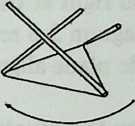
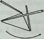
To understand this bootstrap effect, consider first a primitive tensile structure, consisting of two trees, a clothesline, and two poles (Diagram 1.3). The poles slant in opposite directions, and 1.3 the system sketches a contained space.
Next, discard the trees, and fix the ends of the line to the earth, slanting the poles so that their lower ends and the anchor points of the line define a quadrilateral (Diagram 1.4 1.4). Provided the poles are prevented from slipping, this is perfectly stable, and we have framed a tent with no center pole.
If we join the rope anchor points by a third pole, and replace the dotted lines on Diagram 1.4 with additional rope (Diagram 1.5), we shall find that we have a self-sufficient tension/compression system. The rope holds the poles both together and apart. The poles in turn lend shape to the prism-shaped rope network.
Here the reader should convince himself of the properties of this structure by experimenting with a simple model. Three dowels of convenient length (say, 9 inches) will do for the poles. Drive nails or pins into their ends and then tie them together as shown in Diagram 1.5, making the strings two-thirds the length of the dowels. As the last string is tightened, the tension network can be seen pulling the system outward into taut equilibrium. Thereafter the system resists deformation, and if deformed to an extent permitted by the elasticity of the tendons, will tend to restore itself to equilibrium.
The vertex points of this system, 6 in number, may be imagined as points on the surface of an enveloping sphere, since they are equidistant from a point in the center of the tensile prism. Additional members (poles and ropes, or struts and strings) can be so placed as to increase the degree of approximation to a sphere: we can make the system as spherical as we like. (This will be discussed in detail later.) As we do so, we shall find that the poles sketch the sphere’s inner surface, the ropes its outer. In like manner, the stresses on the outer skin of a spherical structure tend to be tensile, and the stresses on its inner skin compressive. And the integrity of the spherical skin as a whole is wholly independent of central support. It is also independent of compressive load-bearing of the kind exemplified in post-and-beam construction or in the arch, since the compressive members are not in contact.
Now, return to the transition between Diagram 1.4 and Diagram 1.5 and note that structural integrity requires either a complete rope-and-pole system or else a partial system plus the earth. Tensional circuits must be completed somehow. Motion pictures of air-lifted geodesic domes show the bottom-edge weaving and wavering until it is set on the ground and affixed there by fastenings.
The rope-and-pole prism shown in Diagram 1.5 is the simplest Tensegrity structure. (Tensegrity = Tensional integrity.) It has no redundant components. All the domes described in this book, notably the numerous “geodesic” variants, exemplify special cases of Tensegrity principles. Their salient continuities are tensional, and their upper portions are not so much supported as lifted by tensional forces.
Unlike the stone arch or the stone dome, such structures are not made stronger by being made heavier. In fact, they can with advantage be made negligibly light in comparison with the tensional forces that bind the components. The one-way tension of terrestrial gravity is replaced by the multi-direction tension of structural members. The system is therefore stable in any position.
Moreover, a tendency to peripheral or local stresses, such as those restrained by the chain round the dome of Saint Peter’s, is supplanted by a multi-directional stress equilibrium. A corresponding multi-directional tension network encloses accidental stresses wherever they arise. There are no points of local weakness inherent in the system.
¶ Appendix to Chapter 1: Tensegrity Prisms
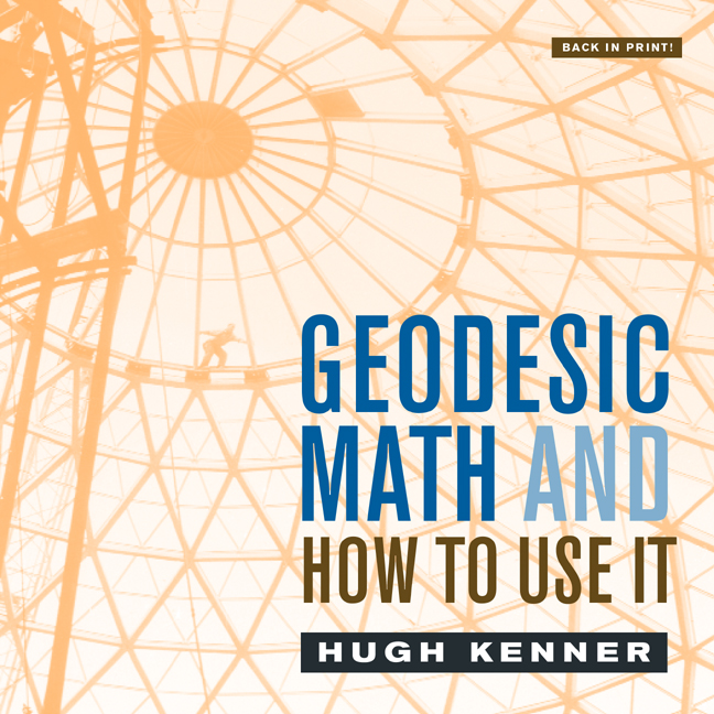
We have noted that the structure developed in Diagram 1.5 is the simplest Tensegrity, consisting of 3 compressive struts and 9 tensile tendons (tendon = the portion of the tensile network between the two adjacent strut ends). It resembles a triangular prism, one end of which has been rotated with respect to the other, thus twisting the quadrilateral sides. One additional strut (Diagram 1.6 1.6) will
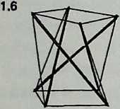
convert the end triangles into squares; a further strut
(Diagram 1.7) will convert them into pentagons; and so forth. It is possible in this way to generate a potentially infinite family of T-prisms corresponding to the prisms of solid geometry.
We may imagine any such T-prism enclosed in a cylinder of height and diameter . The tendons (of length ) outlining the end -gons are called end tendons. There are also side tendons, of length . (In general denotes the number of struts, the number of side tendons, and the number of tendons bounding the end polygons.)
We shall assume that the end -gons are equilateral. If they are equal to one another, the prism is uniform. If they are unequal (though equilateral) the prism is semi-uniform, and would be enclosed by a truncated cone instead of by a cylinder.
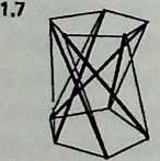
Though they join corresponding vertices of the top and bottom -gons, the struts of any T-prism all lean uniformly, either clockwise or counterclockwise. That is because of the twist referred to above; the top polygon has been rotated with respect to the bottom polygon through an angle called the twist angle (Diagram 1.8). Whatever the height or
diameter of the structure, it can be shown that for a given number of struts, the twist angle is constant and is given by the formula
This remarkable fact[1] makes it easy to calculate the lengths of struts and tendons for any values of , , and .
One way to prove the twist-angle theorem is to use cylindrical coordinates. Diagram 1.9 1.9 shows the coordinate frame with 1 strut , 1 side tendon , and 1 end tendon . Since the end tendon is one edge of the end -gon, it subtends a center angle of . The cylindrical coordinates () of and are thus and , respectively. Point is not located above point but is displaced counterclockwise by an additional angle , the twist angle; its coordinates are .
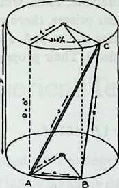
The distances and are strut length and side tendon length , respectively. The standard distance formula for cylindrical coordinates gives: $$s = \sqrt{r_{1}{2}+r_{2}- 2r_{1}{2}\cos{\frac{360\circ}{n}+ \alpha}}+ h^{2}$$ and $$t = \sqrt{r_{1}^{2}+ r_{2}^{2}- 2r_{1}r_{2}\cos{\alpha}+ h2 }$$ Rearranging the first equation, we obtain $$h^{2}= s^{2}- r_{1}^{2}- r_{2}{2}2r_{1}r_{2}\cos{\left(\frac{360{\circ}}{n} + \alpha\right)}$$ and substituting this for in the second equation gives $$t = \sqrt{s^{2}+ 2r_{1}r_{2}\left{ \cos{\frac{360^\circ}{n} + \alpha}- \cos{\alpha}\right}}$$ To find out how this varies, we differentiate it, obtaining $$\frac{\Delta t}{\Delta \alpha}= \frac{r_{1}r_{2}{\sin \alpha - \sin\left(\frac{360^\circ}{n}+ \alpha \right)}}{\sqrt{s^{2}+ 2r_{1}r_{2}{\cos\left(\frac{360^\circ}{n}+ \alpha \right)} - \cos a}}$$ This is messy, but take heart. When the system is taut the tendon length will be minimal, and the derivative above will , signifying no rate of change . At this point the denominator drops out, since it must be the numerator that equals zero. And since the product of the radii cannot be zero, it can only be the functions of that have vanished. So at the equilibrium state, $$\sin\left(\frac{360^{\circ}}{n}+ \alpha\right) = \sin \alpha$$ which is possible if $$\left(\frac{360^{\circ}}{n}+ \alpha \right) = 180^{\circ}- \alpha$$ whence $$2\alpha = 180^{\circ}= \left( \frac{360^{\circ}}{n}\right)$$ and $$\alpha = 90^{\circ}- \frac{180^{\circ}}{n}.$$ The twist angle therefore is a function of alone, and is given by Equation [eq:1-1], above. If we now disregard such physical inconveniences as tendon stretch and deformations imposed by the weight of the structural members, we can use the cylindrical coordinate distance formula to calculate the dimensions of an idealized semi-uniform T-prism. Putting for that is, one-half the diameter we get: $$\text{strut}(s) = \sqrt{r_{1}{2}r_{2}+
2r_{1}{2}r_{2}\sin
\left(
\frac{180}{n}\right)+
h^{2}}\label{eq:1.2}$$ $$\text{side tendon}(t) = r_{1}^{2}+ r_{2}^{2}- 2r_{1}r_{2}\sin \left(\frac{180}{n}
\right ) + h^{2}\label{eq:1.3}$$ $$\text{end tendon}(e) =d\sin \left(\frac{180°}{n}\right). \label{eq:1.4}$$
If the T-prism is semi-uniform there will of course be two end tendon lengths, corresponding to the two diameters.
Example 1.1. Semi-uniform T-prism, 12 inches high, end diameters 6 inches and 10 inches: 5 struts. The equations give 14-inch struts, 12.7-inch side tendons, 3.5-inch tendons for the smaller end, 5.9-inch tendons for the larger end.
Example 1.2. Uniform T-prism, 3 struts, and as high as it is broad. (Thus ): End tendons are sin 60° or 0.86603; struts are 1.39, side tendons are 1.03. Thus for a model 12 inches high, end tendons would be 10.4 inches long, struts 16.7 inches, side tendons 12.4 inches.
It may occur to us to want all tendons equal. In that case we put the right side of Equation 1.4 equal to the right side of Equation 1.3 and rearrange to give : for ,
This proves to be solvable for . For it yields 0, (that is, no height at all), and for it yields a function of , which is not modelable. Thus, while there is an infinite number of regular prisms, there are only three regular T-prisms, corresponding to . ( and are structurally meaningless). Their proportions are:
-
.
Strut:tendon ratio .
-
.
Strut:tendon ratio .
-
.
Strut:tendon ratio .
¶ Spherical Tensegrities
The three-strut Tensegrity described in Chapter 1 is asymmetrical, having triangular ends and rhomboidal sides. It is the simplest member of an infinitely large family of Tensegrity prisms (T-prisms), analyzed in Appendix 1.1. All of these have rhomboidal sides and none can be made omni-symmetrical. Even the four-strut version (T-4 prism) has plane squares at two ends but twisted squares on four sides.
Since we are approaching the design of a dome, we want a Tensegrity whose face patterns, when projected onto a sphere, will divide the sphere’s surface into symmetrically placed zones. The simplest Tensegrity of this kind employs 6 struts arranged in parallel pairs (Diagram 2.1 2.1).
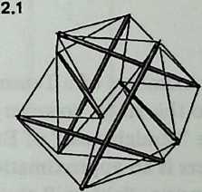
Again the reader should stop and construct a model. There is nosubstitute for experimenting with an actual structure. Use dowels for the struts as before, and make the tendons 0.6 times their length. (For large models, the theoretical ratio is .) When the 24 tendons are in place, it will be found that the parallel strutsare spaced exactly half a strutlength apart, centerline to center-line. We also discover that when two parallel struts are movedtoward or away from each other, the other two pairs move in exact concert. The entire structure expands or contracts symmetrically; it does not bulge here to accommodate a dimple there. The reason the struts will move at all is that the residual elasticity of the tendons is greatly multiplied by the geometry of the system. Elasticity Multiplication to be examined lateris a characteristic inherent in Tensegrities.
This six-strut, twenty-four-tendon Tensegrity has no redundant parts. Each strut is held in place by the cooperative action of a system that comprises twenty-nine other members. When a strut is displaced by application of stress, the whole system undergoes symmetrical modification to accommodate the local movement. The system’s symmetry is not deformed; the system expands as a whole or contracts as a whole. To permit this, each of the eight equilateral triangles rotates about its center; an inward or outward motion of the struts is accompanied by a rotary motion of the tension triangles. Obviously, this ability to respond as a system would be a valuable characteristic of large space-enclosure structures. Ability to respond as a system means that local stresses are being uniformly transmitted throughout the structure, and uniformly absorbed by every part of it. This principle points toward valuable economies in material. Instead of designing every part of the system to receive unassisted whatever loads it may incur, with consequent local accretions of weight and bulk, we may instead design the system on the assumption that local stress will be transmitted throughout its extent, and shared by all its members. The normal state of the system is not a state of rigidity but a state of equilibrium, to which, when disturbed, it seeks to restore itself.
¶ Equilibrium
When the tension members of a Tensegrity are taut, it is in a state of equilibrium. To this state, however stressed, it always seeks to return. Unlike the “straightness” of Euclidean lines, the tautness of tension members is an approximation only. The weight of the cord or cable, however slight, will always curve it slightly; turnbuckles and fastenings have always residual slackness; materials have always residual elasticity. It is impossible to pull any line so tight that it could not, with sufficient effort, be pulled a little tighter. Hence the capacity of the system to absorb displacements and restore itself. Still, for purposes of study and of system design, we can imagine an ideal state of equilibrium in which tendons pull perfectly straight and are perfectly tight, and predict the place every component would occupy if the ideal equilibrium could be realized with actual materials.
Examination of the six-strut Tensegrity discloses four tendons attached to each strut end. By recourse to a chemical metaphor, we may call it a Valence-4 Tensegrity, it is the simplest of a very large family of these. (The T-prism we examined in Chapter 1 has three tendons per strut end and is hence an example of the Valence-3 Tensegrity family.)
The design procedure for a Valence-4 Tensegrity commences from the fact that each strut lies at the bottom of a tensional “valley” whose sides are triangular. Other struts are attached to the apexes of these triangles (Diagram 2.2). Each triangle consists of two tendons plus the strut they share in common. Each pair of tendons, together with the strut, lies in a plane we may call a tensile plane. So each strut lies along the intersection of two tensile planes. (Two intersecting planes, according to projective geometry, suffice to determine the position of a line. This fact may help us understand why the struts tend to stay in place.)
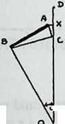
We may now examine the conditions of system equilibrium (Diagram 2.3). Since equilibrium is not a static condition of being “at rest,” but rather the resolution of forces that are pulling in several directions, the way to locate it is to examine the forces that are seeking to disrupt it. In the figure, which is Diagram 2.2 redrawn in a different perspective, is the cross-section of a strut lying at the bottom of a tensile valley ASB. Struts and are being pulled symmetrically outward, left and right, by other tendons in the system. If they were to obey this pull, they would lift strut outward and upward. As this happened, angle , the angle between the two tensile planes that locate strut , would tend to increase.
But other tendons attached to strut are restraining it from moving in this way. They are doing this by pulling it downward and inward. If they were to succeed, strut , in moving downward, would pull struts and inward, and angle , the angle between the two tensile planes that locate strut ,would tend to decrease.
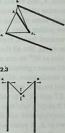
So we can see that the forces in balance are determining angle , the angle between the two tensile planes that locate strut S. Since the system is omni-symmetrical, the pairs of tensile planes associated with each strut will all be at this angle to one another. 2.2 We may call it the dip angle, since the spherical contour of the system here dips inward, incising the polyhedron with a reentrant angle. There is a characteristic dip angle for every symmetrical Valence-4 Tensegrity system. We may intuit, and shall later prove in detail, that if we know the dip angle we can deduce all the system’s component lengths and positions. So our first job is to find the dip angle of the system under consideration.
To deduce the dip angle of the six-strut Tensegrity system, we scrutinize the balance of forces more closely (Diagram 2.4). Concentrate on point , and reflect that in the equilibrium state it stays where it is because all the forces that pull on it are in balance. We may specify some of these forces. The tendons in the tensile plane are pulling point downward and rightward. The rightward and downward forces, represented by the heavy arrows, may be regarded as equal, like all the other sets of forces in the system. They are also at 90° to one another.
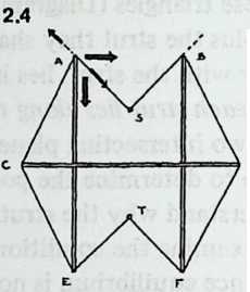
Point does not move rightward because part of the effort of the tendons in the tensile plane is to pull it leftward. It does not move downward because part of the effort of the tendons in the tensile planes and is to pull strut upward. These pulls balance, and it stays where it is.
Now return to the rightward and downward forces represented by the heavy arrows at . A point pulled upon by two equal forces will behave as though it responded to a single force, the angle of which is midway between them. So point responds to a force pulling downward and rightward at 45° to the horizontal and vertical.
Similarly, the tensile plane pulls the point downward and leftward at 45°. Being at 45° to the horizontal, the tensile planes and are at 90° to each other. The dip angle is the angle between these planes. Thus we have found that in the symmetrical six-strut Tensegrity system the dip angle is 90°.
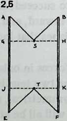
We can now proceed more rapidly. Diagram 2.5 shows the same view of the system as Diagram 2.4, but with strut omitted and with dotted lines and drawn through and . is the separation between struts and , and since the system is symmetrical this will be equal to , the separation between struts and . Moreover, since the dip angles and are both 90°, and . But we know from symmetry that is the midpoint of , and is the midpoint of . Since we have already found that , we see that and must each equal half of . Adding and (or ), we learn that equals half the length of the strut . But we know that corresponds to the separation between the struts and T. And all strut separations are alike. So we have shown that in a symmetrical six-strut Tensegrity system the separation between any two parallel struts is exactly half the length of a strut.
This fact defines the condition of the system when it is in equilibrium. The struts can only be displaced from half-length separation by a force from outside the systeman inquisitive hand, a falling tree, the pull of gravity on strut materials. Once displaced, half-length separation is the condition to which they will seek to return.
It is now a simple matter to calculate tendon lengths for tautness in the equilibrium condition. Diagram 2.6 shows how the pairs of struts are arranged in three mutually perpendicular (orthogonal) planes. In the six-strut Tensegrity system the ends of parallel struts need never be connected; a pair of struts joined by a tendon will always be at a 90° angle to one another. And by symmetry, all twenty-four tendons are of equal length. So there is only one tendon orientation to be considered, and we need only find the length of one tendon.
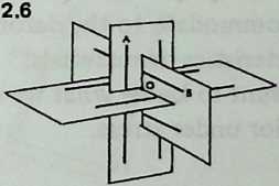
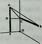
Diagram 2.7, a detail extracted from Diagram 2.6, shows the intersection of the 3 planes, like the meeting of two walls and a floor. Half a strut is painted on one wall; the other half is below the floor. Half a strut is painted on the adjoining wall; the other half is in the far room. Thus and equal half a strut length each. is half the separation between two parallel struts, thus equals 1/4 strut length. Likewise = strut length. Thus . We now have the dimensions we need to solve the right-angled triangle , the hypotenuse of which is a side of the right-angled triangle . The hypotenuse of the latter in turn may be calculated; it is . This is the length of the tendon joining strut ends and .
Thus for strut length = 1, each of the 24 tendons of a symmetrical 6-strut Tensegrity system is , or approximately.
We emphasize once more that this is an ideal Tensegrity system with weightless struts and ideally straight tendons. We have calculated design-center values, to which no actual model, large or small, will ever exactly correspond. In a large structure, say with 10-foot struts, the catenary sag of the tendons will always be effective though it may not be readily measurable. Moreover, strut weight will compress the system somewhat; triangles will rotate and tendons will stretch to accommodate this. And whether the model is made large, with beams and cables, or small, with dowels and string, perfect symmetry will prove impossible of attainment, however carefully dimensions are measured. These facts mean only that an actual Tensegrity structure is never quite in the calculated equilibrium state. We recall, however, from experimenting with a model that it has a unique ability to accommodate departures from equilibrium. It can be designed and constructed as though perfect equilibrium were attainable, and will simply accommodate to the deformities introduced by the physical characteristics of materials.
So we may want to know what we can predict about the system’s behavior under stress.
¶ Elasticity Multiplication
When the system is under stress and hence no longer in equilibrium, the pairs of parallel struts remain parallel but their separation is no longer 1/2 strut length. They have moved either closer together or further apart, and their separation is some new multiple of a strut lengthcall it . As the struts move, the tendons stretch. Their length is no longer , but some greater multiple of a strut length: call it .
To find how and are related, we may redraw Diagram 2.7 and label the distances and not but . (The length of the portions of struts we are dealing with is still ; only the strut separation has changed, from to , so the half-separation shown in Diagram 2.8 is no longer but .) The right-angled triangle now has and for sides, and becomes . Solving triangle with the help of this, we find that , the tendon , is , when and are multiples of strut lengths.
We know the value of when the separation is at the equilibrium condition. Sure enough, if we put for in this equation, we obtain , or (to ten places).
We have obtained a general tendon-length equation for the symmetrical 6-strut Tensegrity:
We are now ready to see what happens if we change the strut separation. Let us try increasing it by 1 percent, a modest increment, well within the stretching capacity of any likely tendon material. We may first define what we might expect to happen.
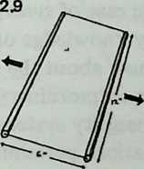
Diagram 2.9 shows a pair of parallel struts 12 inches long. They are joined at both ends by strings 6 inches long, so that the strut separation is half a strut length, exactly as with a six-strut Tensegrity in the equilibrium condition. If we now force them apart an additional 1 percent, the separation will have increased from to , a mere inch. The strings will have no difficulty stretching that far, and we are unsurprised to find that the string length has also increased by the same percentage. To write this compactly, we may use the mathematician’s usual symbol, , for the amount of change. The change in strut separation, , is 0.06 inch; the change in separation expressed as a percentage, , is 1. And the tendon length changes are exactly the same: is 0.06 inch, is 1. So , and .
To find out what happens when we move two parallel struts of a six-strut Tensegrity apart by the same amount, we have only to solve Equation 2.1, putting 0.505 in place of . When we do this we find that , the tendon length, has become . The reader will now see why we calculated the equilibrium tendon length to ten places a page or so back: the difference between the tendon length at equilibrium () and for strut-spacing 1 percent greater than at equilibrium () commences to show up only in the fifth place. The difference is 0.0000102061. In a model with 12-inch struts, separating the struts an additional 1 percent causes the strings to stretch about one ten-thousandth of an inch, which is quite unmeasurable. Dividing separation change by tendon stretch, we obtain not , but .
The elasticity of tensile materials is usually expressed as a percentage of a unit length. Converting the tendon stretch into a percentage, we find that each tendon has stretched percent while the strut separation was increasing 1 percent. So . If we handled the Tensegrity with our eyes shut, imagining that we were holding merely two sticks tied together, as in Diagram 2.9, we should think the tendon material was 600 times more elastic than it actually is. We are encountering the capacity of the system to multiply the elasticity of the tendon material.
We have here a classic case of synergy: behavior of whole systems, unpredicted by knowledge of the parts or of any subset of parts. Nothing we know about the struts and strings could allow us to predict their extraordinary behavior when they are united in a six-strut Tensegrity system.
It follows that calculations pertaining to such a system, taking into account the known characteristics of the materials but presuming the usual methods of assembling them, are certain to be wrong. We might suppose that if the struts were displaced by 10 percent a tendon would break, because our tendon material will not stretch 10 percent without breaking. But a little work with Equation 2.1 will show that a 10 percent strut displacement (from 0.5 to 0.55) changes tendon length by only 0.00102, a mere 0.167 percent. This is only 1/60 of what we might have expected , and well within the elastic capabilities of any tension material we are likely to think of. By analogy, the tensile network hidden in geodesic domes quite defeats all normal calculations of their strength.
The reader will have noticed that when we increased the strut displacement from 1 percent to 10 percent, the ratio of separation change to tendon stretch dropped from 600 to 60. This is generally true of Tensegrity structures: the elasticity multiplication is very great for small displacements (for instance for a displacement of percent), and drops rapidly as displacement increases (about 10 for displacement of 60 percent). Thus Tensegrities are extremely resilient under light loads. A complex Tensegrity model is never quite still, however tightly the tendons are stretched. On the other hand, it stiffens rapidly as loading increases.
We may also wonder what will happen if we push the struts of the 6-strut Tensegrity closer together instead of pulling them apart. The answer is, exactly the same thing. If we decrease the separation by 1 percent, to 0.495, and insert this value into . Equation 2.1, we shall obtain the same tendon stretch as before, and the same ratio, 600. Whether we expand the system or contract it, the tendons stretch, and at exactly the same rate for the same percentage of change. So the system seeks equilibrium exactly as a ball seeks the bottom of a bowl. A graph of the relationship is in fact bowl-shaped; more precisely, parabola-shaped. Any equation such as Equation 2.1, in which one quantity’s variation is affected by the second power of another, will give us a parabola, if we plot points from it (Diagram 2.10 2.2).
The parabola has a theoretical zero point, where it touches the baseline, but this resembles the famous ideal point with position but no magnitude: we can never really say that it is occupied. In the real universe where winds blow, invisible forces tug, and molecules are in ceaseless motion, a Tensegrity will no more quite settle down than will anything else: there will always be minute motions, tiny strut displacements at the order of magnitude where elasticity multiplication is truly enormous and compensating forces have enormous advantage. The parabola’s zero point is that ideal condition of rest which nothing real ever attains, and about which a Tensegrity in particular dances an eternal jig of pre-Socratic derision.
¶ Complex Spherical Tensegrities
The simplest spherical Tensegrity, the six-strut Valence-4 version with struts in three parallel pairs, has occupied us for many pages. There are several reasons for understanding it in considerable detail. (1) Tensegrity structures and the geodesic domes of which they supply first-approximation stress diagrams, have been shunned by many investigators as unduly mystifying. It is worthwhile becoming convinced that their behavior yields to rational analysis. (2) While dodges such as calculus would have shortened the work, they can mislead unless we are sure we understand the phenomena we are using them to describe. Simple mathematics and experience of the directions in which strings pull taut will suffice if we are patient. (3) The analysis has turned up some principles that will help us with more complex structures. These include:
-
the property of behaving as a system in response to local events,
-
the normal state as an ideal equilibrium about which observable behaviors oscillate,
-
elasticity multiplication, a special case of synergy,
-
the parabolic curve as a graph of system behavior,
-
the value of the dip angle as a point of analytic attention.
¶ Great Circle Tensegrities
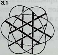
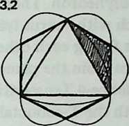
Examining the symmetries of the six-strut Tensegrity, we may think of surrounding it by three intersecting hoops, located like the equator, the Greenwich meridian, and the 180° meridian (Diagram 3.1 3.1). Each of these hoops a great circle, or geodesicpasses through both ends of one pair of parallel struts, and the three of them contain the system symmetrically. They resemble the great circles of the regular octahedron (Diagram 3.2 3.2), each of which contains four octahedron edges. We may wonder if there are Valence-4 Tensegrity equivalents to other great-circle polyhedra. There are; but their number is severely restricted.
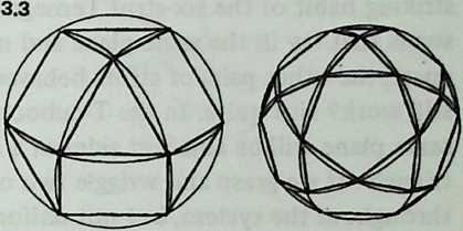
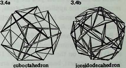
Still, they have a great deal to teach us. We need polyhedra whose edges, projected onto a sphere, make great circles. We also need exactly four edges at each polyhedron vertex. There are just two polyhedra that will fulfill these conditions: the cuboctahedron and the icosidodecahedron (Diagram 3.3 3.3). Tensegrity equivalents to these polyhedra are shown in Diagram 3.4.
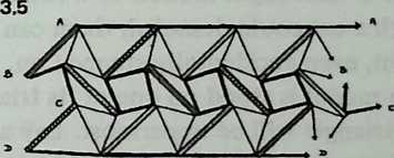
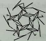
Once again, make models: preferably of both structures, but at least of the simpler (cuboctahedron). It is worth a little trouble. The Tensegrity cuboctahedron (abbreviated T-cuboctahedron has twelve struts, arranged in four groups of three. Paint each group a different color before assembly. Use 1/4-inch or 3/16-inch dowel and make the struts 12 inches long. Drive pins into the dowel ends to anchor the tendons. Use thin, tough cordage: braided nylon fishline is excellent. (Avoid monofilament nylon, in which it is difficult to tie a nonslipping knot.) Diagram 3.5 shows a net diagram, and tendon lengths are indicated. Do as much as possible flat on the table; then join the indicated points, to close up the sphere.
Diagram 3.6 shows part of the net diagram for the T-icosidodecahedron. It uses thirty struts in six groups of five (six colors).
The T-cuboctahedron when completed should contain four equatorial triangles; the T-icosidodecahedron should contain six equatorial pentagons.
The T-cuboctahedron resembles the regular cuboctahedron in two principal ways. (1) Its struts describe four symmetrically placed great circles. (2) Its tendons outline the six squares and eight triangles of the cuboctahedron’s faces.
We immediately notice two points of difference. (1) Whereas the cuboctahedron has six edges around each great circle, the T-cuboctahedron has only three struts. (2) The square and triangular faces outlined by the tendons do not abut on one another as do the faces of the polyhedron. They are separated by diamond-shaped segments, each with a strut lying along its long axis and with two other struts facing each other end-to-end across its short axis. These differences from the parent polyhedron are general characteristics of Valence-4 Tensegrities.
Experimenting with the T-cuboctahedron, we may collect some observations about its behavior under stress. We remember a striking habit of the six-strut Tensegrity: when we grasped two struts that lay in the same plane and moved them together or apart, the other pairs of struts behaved in exact concert. Will this still work? Not quite. In the T-cuboctahedron, two struts in the same plane will be adjacent sides of a circumferential strut triangle. If we grasp and wriggle two of these, action will occur throughout the system, but not uniformly. Watch the gaps between adjacent strut ends of the circumferential triangles. These will open and close as struts displace themselves. The gaps within which lie the two struts you are grasping will barely alter. Others, remote from the application of stress, open and close markedly. In general, disturbance is relayed to portions of the system far from where it entered. A ninety-strut 40-foot Tensegrity sphere erected at Princeton University in 1953 was struck by a snowplow at a point near the ground and exhibited component failure (a bent strut) high up on the other side, just 180° from the point of impact. In general, because stresses are diffused, component failure is rare. Light models of wood and string that look as though a cat could demolish them can be kicked, bounced, thrown, even accidentally stepped on, without damage.
If a model is stood on one of its triangular sides, another equivalent triangle will be uppermost. Lay a weighta heavy bookon this upper face. As the model compresses, it will rotate. The equatorial strut triangle neither bulges nor shrinks; it simply revolves. Others are deformed in complex ways. The net effect is compression of the sphere into an oblate spheroid, but without increase in diameter. The rotation of the equator takes up the forces that might be expected to expand it.
The direction of rotation Under contractive stress is determined by the handedness of the system. Most Tensegrity systems exist as right- and left-handed mirror pairs; a particular model is either one or the other. It is easy to see (Diagram 3.7) that the three struts 3.7 which rise from vertices of a triangular base can sketch either a clockwise or a counterclockwise rotation. Under compressive stress, these struts swing away from one another, either clockwise or counter-clockwise, according to the handedness of the system. The three struts angling downward from a triangular summit also swing away from each other, but since the upper cone is inverted with respect to the lower, their movement with respect to the equator is in the opposite direction from that of the base struts. Thus each equatorial strut is pulled both clockwise and counter-clockwise simultaneously; the stresses cancel, and the equatorial struts move neither out nor in. Thus the size of the equator (as we have noticed already) is unchanged. Instead the equator, and with it the whole system, is carried bodily around in the direction of rotation of the base struts. The only motionless zone is the base triangle, which is fixed to the floor, the tabletop, or the earth.
The six-strut Tensegrity of Chapter 2 is an exception to the general principle of right- and left-handedness. It has no handedness, hence no ring of cancellation, and so behaves with perfect symmetry throughout. All twelve of its vertices are displaced alike.
¶ Dip-Angle Calculations
We next require a general procedure for calculating the dimensions and component lengths of spherical Tensegrities more complex than the six-strut one we have analyzed. The key to this, as before, is the dip angle.
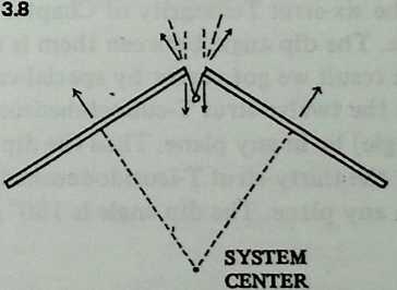
Examining the six-strut structure in Chapter 2, we discovered that the dip angle between parallel struts was necessarily 90°. Diagram 3.8 3.4 shows how to extend this reasoning. It depends on something we can readily observe by inspecting a model, that any strut we may concentrate on is staying where it is because two opposed forces are balanced out. The two tensile planes at whose intersection it lies are bounded by four tendons whose net effort is to pull it straight outward, away from the center of the system. It is anchored at its ends, however, by tendons whose net effect is to pull it straight inward, toward the center of the system. These forces can be diagrammed right at the end of the strut, where all tendons are attached; Diagram 3.8 3.4 represents them by light arrows. The tendons in the tensile plane align themselves midway between these forces.
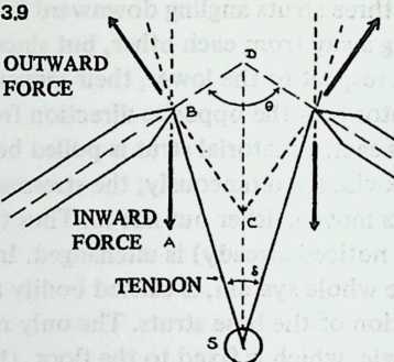
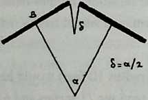
Diagram 3.9 [fig:3.9] shows how the situation would look if the struts were extended until they touched. They enclose an angle we may call 0. The rest is simple geometrical reasoning, shown with the diagram. We conclude that whatever the angle, at which two struts meet, the dip angle will be
These two struts are sides of a regular polygon which lies in the plane of a great circle round the models we have examined, but which may lie in a lesser circle plane round Tensegrities we shall encounter later. In either case, the angle between two adjacent struts is the interior angle between any two sides of a regular polygon with sides. This is . Equation 3.1 tells us that the dip angle is 90° minus half this, or . Simplified, this gives us a compact alternative form for the dip-angle equation:
So we have only to divide 180° by the number of struts in one plane of a Tensegrity sphere (otherwise put, the number of struts round a great circle or lesser circle) to obtain the dip angle between any two of these struts. The six-strut Tensegrity of Chapter 2 has two struts in each plane. The dip angle between them is thus 180°/2, or 90°, the same result we got earlier by special-case reasoning. In the twelve-strut T-cuboctahedron, three struts (an equilateral triangle) lie in any plane. Thus the dip angle is 180°/3, or 60°. In the thirty-strut T-icosidodecahedron, five struts (a pentagon) lie in any plane. The dip angle is 180°/5, or 36°.
¶ Calculation of Remaining Dimensions
We shall now see how the dip angle can be used to calculate all the remaining dimensions of a Valence-4 Tensegrity sphere.
It is convenient to call the strut length 1 and express all other dimensions in strut lengths. If calculation shows that a certain tendon length is 0.523, this means it is strut length. If we are using 8-foot struts, this tendon will be , or 4.184 feet or 50.2 inches.
For model-building, we normally start with known strut lengths, anyhow. For larger structures, we are more likely to start with a desired diameter. No problem. Equation 3.5, below, relates radius to strut length and so gives us access to all the other dimensions, even when the size of the structure we want to build and its geometry are the only two things we know. Proofs of all equations in this chapter are given in the chapter appendix. Elementary geometry and trigonometry suffice to yield all of them.
-
We obtain dip angle $$\delta = 180^{\circ}/n,\label{eq:3.2}$$ where = number of coplanar struts around the structure.
-
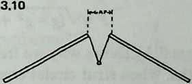
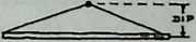
We derive the gap . The gap (Diagram 3.10) is the linear
distance between the ends of two adjacent struts on a greater or lesser circle. $$g = sin^{2}(\delta/2).\label{eq:3.3}$$
-
We next find the dip. The dip is the median of a tensile plane: the distance (Diagram 3.10) from a strut end to the mid-point of the strut that crosses beneath it. Its symbol is , and $$d = \sin/2(\delta/2).\label{eq:3.4}$$
We pause to notice that tendons which simply follow the dip, joining the ends of adjacent struts to the midpoint of the strut passing below, will suffice to make a stable structure with no othertendons whatever. In these center-connected Tensegrities, whose only tension members are little V-shaped slings, the tension network is no longer optically continuous but must be traced in part through the struts. This is not a recommended method of construction because it imposes a bending load on the struts. It is a good way to analyze certain features ofTensegrity construction. It particular, it draws our attention to the fact that the dip is the crucial parameter. When the dip slings in such a model are correctly dimensioned, the gaps and strut angles will automatically adjust themselves into the equilibrium state, and all struts around any great circle or lesser circle will align themselves in a common plane.
-
We now obtain the radius, . This means the radius of the circumsphere: a sphere into which the Tensegrity would exactly fit, all its strut ends touching the spherical envelope. Or it is the distance outward from the center of the system to the end of any strut. The equation is brief: $$r = \sqrt{\frac{(1 +3g)}{16g}}\label{eq:3.5}$$
This gives us the radius expressed in strut lengths. Should we wish to design a sphere of given radius , then the strut length is, of course, .
-
Our next step is to obtain an arbitrary quantity . Its whole purpose is to simplify the tendon-length equations by working out separately a portion common to each of them. $$P = \sqrt{\frac{g-g^{2}+ 1}{4}}\label{eq:3.6}$$
-
Diagram 3.11 shows why we frequently need two different tendon lengths. When strut circles cross one another at 90° angles, tendon lengths are equal. When they cross at some other angle, long and short tendons alternate around each strut. To find the two lengths, we shall need the angle at which the planes bounded by strut circles cut one another: more precisely, we need the cosine of this angle. The axes of great-circle and lesser-circle planes are a polyhedron’s axes of symmetry, and since all regular and semi-regular polyhedra have either octet or icosahedral symmetry, there are only three possible values for :
-
Circle axes at 90°.
-
Octahedral symmetry, circle axes at .
-
Icosahedral symmetry, circle axes at .
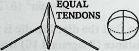
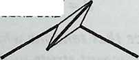

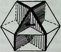
Diagram 3.12 shows the simple case of the cuboctahedron. It is 3.12 octahedrally symmetrical, and we may expect cos t to be 1/3. That is because the angle at which great-circle planes intersect is the dihedral angle of a tetrahedron, or 70.5288°, the cosine of which is 1/3. Tendons calculated by using this value in Equation 3.7 and Equation 3.8, below, will be taut and the model symmetrical, with circumferential struts aligned in common planes.
We pause to note one complication, more likely to affect the model-builder than the dome engineer: the essentially static mathematics of polyhedra will not always coincide with the dynamics of a Tensegrity. This is apt to show up whenever we encounter edges that lack a triangular face on at least one side. For instance, the small rhombicosidodecahedron, a Valence-4 polyhedron, consists wholly of intersecting lesser circles which cut it into square, pentagonal, and triangular faces. It yields a handsome Tensegrity sphere of sixty struts. Since the twelve lesser circles are icosahedrally coordinated, is , and Equation 3.7 and Equation 3.8 will yield long and short tendon lengths. If we construct the model, however, we shall find (Diagram 3.13) that each strut has a triangular face along one side of only one end. The triangle pulls the associated square face into a diamond shape in such a way as to make all strut intersections equiangular. To make the model symmetrical we must refigure the tendons as though were 0, and all tendons of equal length. Methods of foreseeing such effects are of such limited application as not to seem worth the space required to expound them. Check all Tensegrity predictions by building models.
-
-
We may now figure the long and short tendons, and .
t_{1}= \sqrt{p^{2}+ (g/2)^{2}+ (Pg \cos t)}\label{eq:3.7}$$ $$t_{2}= \sqrt{p^{2}+ (g/2)^{2}- (Pg \cos t)}\label{eq:3.8}$$ When the great-circle axes cross at $90^{\circ}(\cos t = 0)$, we have a single tendon length $t$, obtained very simply: $$t_{1}= \sqrt{\frac{(g+1)}{4}}. \label{eq:3.9}
To illustrate this latter situation, consider the six-strut Tensegrity of Chapter 2. It has two struts in each plane, so by Equation 3.2 the dip angle is 180/2, or 90°. The gap, by Equation 3.3, is , or 0.50. This is another way of stating what we learned before, that the separation between parallel struts is half a strut length. And the tendon length, by Equation 3.9, is (0.5 + l)/4, or 0.6124, which checks with what we obtained by geometrical reasoning. Table 3.1 illustrates the other two symmetry cases, deriving step by step the dimensions given in Diagram 3.5 and Diagram 3.6 for the T-cuboctahedron and the T-icosidodecahedron. A sophisticated pocket calculator makes such computations so simple it is easy to become addicted to their multidecimal precision. Pause to reflect what it is we are calculating. We are describing to a high degree of accuracy the equilibrium state of an ideal Tensegrity sphere built of weightless materials. In the equilibrium state so envisaged, the tendon network pulls only against the ideal incompressibility of the compressive struts. In a real structure the one-directional tensile field of earth’s gravity pulls through the multidirectional tensile field of the structure, imposing flattenings and compensatory rotations, as described earlier in this chapter. Tendons, however tightened, will describe catenaries, not straight lines, and two tendons will not meet at a point but at a fastening of measurable size. Moreover, no one but a model-builder or a sculptor is likely to construct a complete sphere. Tensegrity domes are quite practical, and inspection of spherical models will suggest the simplicity of equatorial truncation. Groundlevel anchor points for certain tendons, and the thrust angles of half-struts embedded in the ground, are easily determined. Since with the aid of a few strategically placed turnbuckles it is relatively easy to lengthen or shorten tendons in the field, the designer may safely calculate dimensions from the equations, compensating where necessary for modes of fastening, and make adjustments on the actual structure.
| T-Cuboctahedron | T-Icosidodecahedron | |
|---|---|---|
| 3 struts per great circle | 5 struts per great circle | |
| Dip angle | 180^{\circ}/3 = 60^ | 180^{\circ}/5 = 36^ |
| Gap | ||
| Dip | ||
| Radius | ||
| Long tendon t_ | ||
| Short tendon t_ | ||
| Thus, a model using 12-inch struts would require tendon lengths of 18.2 cm. and 15.7 cm. and would have a radius of 7.9 inches.[2] | Thus, a model using 12-inch struts would require tendon lengths of 16.6 cm. and 15.3 cm. and would have a radius of 11.3 inches. | |
| A 10-foot-diameter structure (radius 5 feet) would have struts 7\sfrac{1}{2} feet long and use tendons 54 inches and 46.8 inches long. | A 20-foot-diameter structure (radius 10 feet) would have struts 10.89 feet long and use tendons 71 inches and 65.6 inches long. |
¶ Appendix to Chapter 3: Derivation of Tensegrity-Sphere Equations
Why the dip angle assumes the value it does, we have discussed in the text. This appendix shows in detail why the gap, dip, radius, and tendon lengths necessarily follow from the dip angle. The reader who is content simply to use the equations is at liberty to skip these proofs.
Diagram 3.14 shows two struts, with tendons at the ends making a dip angle , and radii from their centers to the center of the system, where they make the center angle . Since all the center angles in the system will total 360°, for . But from Equation 3.2, .
We move on to Diagram 3.15, which shows half a strut , two radiiBO and with the angle between them, a half dip angle, , and a half gap, . Angle and Angle are both 90°, and is the dip.
We have shown that ; hence Angle , and Angle . Since , triangle is isosceles, and Angle . But since Angle , Angle , which is a straight line minus both Angle and Angle , must be 90°. Thus is a right-angled triangle, and . Calling a strut length 1, . But since Angle , and Angle = Angle = (180° - )/2, Angle . Thus: $$dip = \sin/2 (\delta/2).\label{eq:3.4b}$$ The gap equation follows readily. is half the gap, and Angle is 90°. So in the right-angled triangle , where the angle at is , . Thus the , or , which simplifies to $$gap = \sin^{2}(\delta/2).\label{eq:3.3b}$$
To derive the radius, we redraw the previous diagram (as Diagram 3.16) inserting () the circumsphere radius we wish to find. It is the distance from the center to the tip of a strut. Various things we know already are written beside the diagram. We see immediately that in the right-angled triangle , Side . We also see that in the isosceles triangle , Side . Thus . Finally, in right-angled Triangle , the hypotenuse . Substituting into this the value we have just obtained for , we get . Since and , this reduces to 3.16 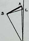
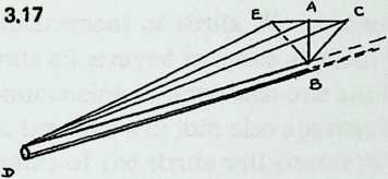
Diagram 3.17 and Diagram 3.18 show how the equations for the tendon lengths are derived. Diagram 3.17 is a perspective drawing showing half a strut, the gap, the associated dips, and the two tendons. We have also drawn a perpendicular, , from the strut to the midpoint of the gap (thus ) and joined to .
The working is now fairly obvious. In right-angled Triangle , we know and and can calculate . In the right-angled Triangle , we know that , and having derived can calculate . This is the quantity of Equation 3.6.
We then turn to Diagram 3.18, in which and are each and . In Triangle we thus know two sides and the cosine of the included angle, and the standard formula yields us Equation 3.8 for the short tendon . The equation for the long tendon is then derived from the fact that .
¶ Tendon System Minima
Commencing with a clothesline and two poles, we have considered in turn elementary Tensegrity systems (Chapter 1), the six-strut spherical Tensegrity (Chapter 2), and twelve-strut and thirty-strut spherical Tensegrities (Chapter 3), the configurations growing ever more suitable for slicing off to yield practical domes. We are gradually deriving the structural principles of the geodesic dome from the Tensegrity sphere, of which it is a special case. The reader will reap the benefits of this approach when he arrives at the geodesic dome prepared to think of its sustaining structural continuities instead of assuming that rigid framing members exist to bear the weight of other rigid framing members, like studs in a frame house or bricks in a wall.
In two more steps we shall have arrived at domes in which things are bolted together instead of slung from cables. The reader anxious to get there may skip the present chapter, which refines our understanding of Tensegrities by describing in another way the forces they contain. The reader who finds Tensegrity independently fascinating is invited to tarry.
¶ Six-strut Tendon Minima
In Chapter 2 we derived the equilibrium condition of the six-strut Tensegrity by concentrating on the sets of opposed forces whose compromise causes the dip angle to settle where it does. In Chapter 3, by a generalized version of the same reasoning, we arrived at a simple equation for predicting the dip angle of a multi-strut Tensegrity sphere. We also learned that the dip angle governs all the other dimensions of the Valence-4 Tensegrity systems, so that knowledge of the dip angle enables us to calculate them.
It might have occurred to us to approach the initial problem in Chapter 2 differently. We might have reflected that when we build a six-strut system we pull all the tendons tight, so tight that they cannot be pulled any tighter. It appears, then, that when the Tensegrity is in equilibrium the total length of the tendon system is minimal. This deduction is reinforced by our discovery that however we disturb the system we stretch the tendons; hence in equilibrium they must have been as short as possible. If we could arrive at the conditions for minimum tendon length, we should have another way of calculating the critical dimensions of the system.
We have seen what governs change in tendon length: it is displacement of struts. We can imagine the three pairs of parallel struts all arrayed in space at some large separation, and then commencing to approach one another symmetrically. The ends the tendons will join also approach one another. Eventually the centers of the struts will cluster at the center of the system. But some time before that happens, the ends the tendons will join will have come as close together as they are going to and will have started to move apart once more. It is that moment of maximum proximity (minimum separation) that we want to fix.
When we came upon elasticity multiplication in Chapter 2, we discovered (Equation 2.1 [eq:2.1]) that whatever the separations between parallel struts, the distance each tendon will span is . This equation is not linear (Diagram 2.10 shows that it is represented by a parabola). The rate at which the tendon length changes, levels off slowly until for a critical instant there is no change at all (the zero point of Diagram 2.10; the tendon minimum we are pursuing). Then the rate of change increases once more, slowly at first, then faster. Anywhere along the parabola in Diagram 2.10, a steep slope designates rapid change, a shallow slope slow change. At the elusive instant of horizontality (zero slope) the rate of change is zero.
None of this is news to the freshman calculus student, who learned on the first day of class that the rate of the change going on in an equation is described by the derivative of the equation, and a few days later was able to write the derivate of . It is . When the quantity is minimal it has momentarily ceased to change: its rate of change (hence its derivative) is zero. This will happen when , that is, when .
This means that when the distance between parallel struts in a symmetrical six-strut Tensegrity is , the distances to be spanned by the tendons, and hence the lengths of all tendons, are minimal.[3] This half-strut-length strut separation agrees with what we learned in Chapter 2 by a different chain of reasoning. To learn the length of this minimum tendon, we have only to return to Equation 2.1 and write for . $$t =\sqrt{(1/2^{2}- 1/2+ 1)/2}.$$ Then , which also agrees with the result we obtained in Chapter 2.
So for a symmetrical six-strut Tensegrity system the assumption that the dip angle will be 90° and the assumption that the tendon system will be of minimum length yield exactly the same results.
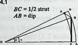
It is not difficult to show that this principle holds true of complex spherical Tensegrities as well. Consider Diagram 4.1, which shows half a strut with its midpoint at a distance from the center 0 of the system. is the dip, which terminates at the midpoint of another strut shown in cross section at . Since all strut midpoints are equidistant from the center, . Angle , bounded by , is obviously , where is the number of struts round a circle. The angle is half the angle subtended by a strut at the center of the system and will increase as the strut is pulled in toward the center. As this happens, point will also move in, since all struts move uniformly, and the dip will change. Hence the angle tells us how far each strut is from system center and gives us an alternative way of defining the equilibrium state.
We can define the dip as a function of angle :
Differentiated with respect to , this gives
Setting this equal to zero and discarding two irrelevant possibilities, we find that for minimum tendon length,
If we now substitute this for in Equation 4.1, we discover after some tedious routine work that when the tendon length is minimal, the dip is , which a glance at Equation 3.4 will show us is exactly what we arrived at in Chapter 3 by the dip-angle method.[4] And all other dimensions follow from that of the dip.
So when any complex spherical Tensegrity is at its equilibrium state, all tendons, and hence the total tendon system, will be of minimum length.
This tells us rigorously what we may have intuited, that we bring a Tensegrity to its equilibrium state by pulling everything as tight as possible. Thereafter any outward or inward force, in attempting to make the system larger or smaller, must also strive to make the tendons longer and will be inhibited by their restoring elasticity. Elasticity multiplication will permit the system to yield more than we might expect, but it will always seek to restore itself to equilibrium.
¶ Geodesic Subdivision
We have been increasing the number of struts in a spherical Tensegrity system, from six to twelve to thirty. The systems have been growing more spherical, because they have more vertices, closer together, and the chords connecting these vertices (struts and tendons) are less and less different from arcs. In addition to making the spherical surface smoother, and hence easier to equip with a weather-break, the progressive shortening of structural members tends to make large structures increasingly practical.
Still, we seem to have reached a limit. The inventory of uniform polyhedra which are both bounded by great circles and equipped with four edges per vertex is exceedingly short. In fact, we have now employed the only three: the octahedron, the cuboctahedron, the icosidodecahedron, corresponding respectively to the six-strut, twelve-strut, and thirty-strut Tensegrity spheres. We might explore existing Zesser-circle systems; indeed we have briefly discussed the small rhombicosidodecahedron, which will make a sixty-strut Tensegrity sphere. If we make this model, or even diagram it, one disadvantage appears immediately: it has no appealing natural lines of truncation. Slicing it on the plane of a lesser circle, we acquire two relatively useless pieces: an extremely shallow saucer, and a 7/8 sphere like an inverted goldfish bowl. Another disadvantage is longer-range: we have no reason to expect the inventory of Valence-4 lesser-circle polyhedra to last much longer than the great-circle series did.
If we are not to be constantly frustrated by the nonexistence of the sort of polyhedra we want, we shall need a way of devising new ones to our specifications.
This possibility does not collide with the geometer’s contention that polyhedra come in small, finite sets. The sets are small because the geometer stipulates that faces of the same shape must be exactly alike. This imperative is rather aesthetic than structural, and once we relax it, we shall find at our disposal literally infinite arrays of nearly uniform polyhedra, as multi-edged and as elaborately faceted as we may wish. We acquire them by systematically subdividing the faces of existing polyhedra.
Diagram 5.1 shows a regular octahedron, having eight equilaterally triangular faces. Diagram 5.2 shows each face of the octahedron divided into four smaller triangles, by simply connecting the midpoints of the edges. These thirty-two small triangles are also equilateral, but the figure does not look promising as a way of generating anything spherical. The reason, of course, is that the vertices and mid-edge points of the octahedron are at different distances from its center. If we call the center-to-vertex radius 1, the center-to-mid-edge radius is only V2/2, or 0.7071.
But there is no reason at all why the twelve vertices that lie on the octahedron’s midedges cannot be pushed out until they are as far from the center as the eight vertices that coincide with the octahedron’s vertices. The radii to all twenty vertices will then be identical , as if the vertices all lay on the surface of a sphere, and the edges that connect them will be chords of that imaginary sphere.
Diagram 5.3 shows what this would look like. Notice that we are not envisaging spherical triangles. The sphere implied by the drawing is nothing but a handy way of reminding ourselves that all vertex points are at a uniform distance (called 1) from the center of the system. The lines that bound the triangles are straight, not curved; chords, not arcs.
We can concentrate now on one octahedron face. Diagram 5.4 shows what has happened to it. The midpoints of the sides have been pushed out until their distance from the center is the same as the distance of from the center . It is clear that the triangle is equilateral, since it still corresponds in shape to the equilateral . In moving out, however, its edges have grown larger, by the same geometry which gives a larger image when the screen is farther from the projector. But has not grown by so much, since its upper end is still anchored at ; it is like an image projected on a tilted screen. The same is true of . So the top triangle, , is not equilateral but isosceles.
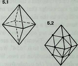
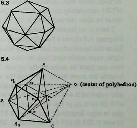
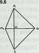
If we want data on this polyhedron, we thus have two edge lengths to calculate. Diagram 5.5 shows a way to go about it. Two applications of Pythagoras’s theorem will give us those isosceles legs, and the knowledge that similar triangles are similar in all respects will give us the sides of the equilateral central triangle.
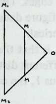
So we have devised a polyhedron with triangular faces. Eight of them are equilateral, with sides equal to the polyhedron’s radius (= 1). Twenty-four are isosceles, with bases equal to 1 and two legs equal to . We obtained this by dividing each edge of the octahedron in two. We call this process a two-frequency division of the octahedron, and we call the resulting polyhedron a two-frequency octahedron ( octa for short).
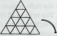
There is no theoretical limit to this process of frequency subdivision. Diagram 5.6 shows how to generate one face of a four-frequency octahedron ( octa) and Diagram 5.7 shows the polyhedron we obtain. Diagram 5.8 lists edge lengths for the sixteen triangles we derive from each octa face. (Ways of calculating them will occupy us later.) They are of four different shapes: one equilateral () at the center; three isosceles () at the comers; three more isosceles () abutting the center; six scalene () completing the edges. Since this pattern is completed eight times to close the polyhedron, the octa has 128 triangular faces.
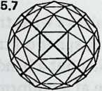
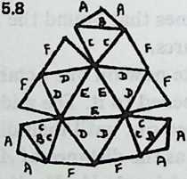
There is no reason to restrict this procedure to the octahedron. Diagram 5.9 shows a four-frequency icosahedron ( icosa). Since the icosahedron has twenty triangles to the octahedron’s eight, each subdivided face has less curvature to supply and therefore can itself be more gently curved. Thus the different edge lengths are more nearly alike and the small triangles more nearly equilateral. The most distorted triangles, the corner ones, have side ratios of in the octa () and side ratios of 0.29 to 0.25 in the icosa (1.16 to 1). The greatest discrepancies in edge lengths ( and ) are for the octa (1.8 to 1) and for the icosa (1.28 to 1).
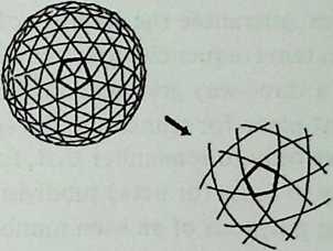
It is clear that an icosa yields less jerky polyhedra than an octa. It is also clear that, octa or icosa, the higher the frequency, the smoother the arcs and the less the tiny triangles differ.
The acute reader will have been wondering what happened to our quest for Valence-4 polyhedra to generate Tensegrities. In the polyhedra we are learning to generate, six-way vertices preponderate, relieved only by twelve Valence-5 vertices when we start with the icosa, and by eight Valence-4 vertices when we start with the octa. Courage. The Tensegrity fan has a simple recourse, illustrated in Diagram 5.10. He has only to omit every other stripe in each of three directions on the face triangle, and lo, the Valence-4 vertices appear.
Following the usual Tensegrity rule of skipping every other vertex, we may insert 120 struts into six pairs of parallel lesser circles, ten struts per circle. The dip angle will be 180°/10, or 18°, and other dimensions may be computed as usual. We have only to remember that the radius yielded by Equation 3.5 is that of a lesser circle and divide it by the cosine of the lesser circle’s “latitude” above the equator to obtain the radius of the actual sphere. The surface pattern of the four-frequency Tensegrity icosa ( icosa) is determined by twelve pentagons, each surrounding a vertex of the icosahedron from which we started (such vertices are always surrounded, not occupied, so we do not encounter the problem of devising a five-way Tensegrity intersection). Five triangles abut the five sides of each pentagon, and five hexagons touch its vertices. Since all twelve lesser circles are alike, all struts are the same length. The six different edge lengths into which we factored the icosa face in executing the original breakdown impose no complication because most of them disappear, and for Tensegrity purposes it is unnecessary to compute them at all. (This won’t hold true of higher-frequency subdivisions.)
It is obvious that by extending this principle, we can generate spherical Tensegrities as complexly multi-strutted as we like. This means in practice that no matter how large a domical structure we may want to build, we can still use struts conveniently short and light. It will exhibit (assuming an icosa generator) a surface pattern of twelve pentagons per complete sphere, plus assorted triangles and hexagons. The triangles, increasingly numerous at higher frequencies, guarantee the stability of the structure. Lesser circles (and at certain frequencies great circles also) will run round the sphere in a three-way grid, and any circle we choose will supply a convenient plane for truncating the sphere to produce a dome.
We have only to remember that, for Tensegrity purposes, the frequency of icosa (or octa) subdivision must always be even, producing polygons of an even number of sides and permitting us to skip every other vertex when we insert the struts. If it is not a Tensegrity that we contemplate, but some other kind of geodesic structure, the restriction to even frequencies does not apply.
¶ Rigid Tensegrities
We are now ready to make the transition from Tensegrity structures to geodesic domes. We commence by noticing that the polyhedra we have been generating with the aid of frequency subdivision have one particularly useful property. As the frequency of subdivision increases and the number of edges grows more numerous, the surface of the sphere-like form also grows smoother.
Analogously, in Tensegrity spheres, gaps and dips grow less and less obtrusive. We shall now see how this fact can be put to use. Tensegrity polyhedra, we remember, are constantly interrupted by the sharp incisions of the dip angles. Whenever a running mouse comes to the end of a strut, it must leap the gap to the end of the next strut. How long a gap, we know from Equation 3.3. How deep a gap? How far down from its middle to the strut that passes below? This depth is a function of both gap and dip; as Diagram 6.1 shows,
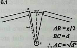
But we know from Equation 3.3 and Equation 3.4 that gap and dip both diminish as the dip angle diminishes; and we know from Equation 3.2 that the dip angle diminishes as the number of struts around a great circle or a lesser circle increases. So increasing the number of struts around a circlewhich is what we are doing when we increase the frequencyboth shortens the gap and diminishes its depth.
This means (Diagram 6.2) that as we increase the frequency 6.2 each gap narrows, and as it does so the strut that passes beneath it moves outward from the center, closer to the surface of the sphere. If it moves outward until the depth of the gap is just equal to the thickness of the struts, it will be so situated as just to touch the bottom edges of the upper struts (Diagram 6.3). By this time the gap will be extremely narrow, and a very little extension of the ends of the upper struts will ensure that they too will touch.
Let us suppose that the system is made.of wood. We can cut the ends of the upper struts so they meet squarely, and we can bevel the upper edge of the lower strut so it fits snugly under them. We may also remember from Chapter 3 the option of replacing the large tensional diamond by a little sling that follows the lines of the dip. Diagram 6.3 shows it embedded in the wood, but it may easily be replaced by a couple of bolts. Tightening the nuts will draw everything together.
Now, note carefully: When we commenced this process, the rest of the system was tending to pull all three components apart. Now that they are touching each other, this is still true. The two upper struts are not in compressive contact: if released, they would pull apart. And they are not resting on the lower strut: if released, they would move outward and away from it.
The bolts and nuts are quite literally serving to draw the elements together. They are performing the function of the tension members in the original Tensegrity.
Repeat this throughout the domical structure, and we have an array of interlaced polygons, weaving alternately above and below the polygons they cross, and bolted at the crossing points. They outline pentagons, hexagons, and triangles and make a sturdy domical structure with no noticeable flexion (Diagram 6.4).
Having developed this structure from Tensegrity principles, we know about the tensile forces that are holding it together. Trace- able through the bolts and the wooden beams, they form a tensional continuity, resembling the surface tension of a liquid sphere in being concentrated on the outer surface of the polyhedron.
But a casual observer of the structure would soon commence studying the joints, and seeing what is diagramed in Diagram 6.3 he would suppose that the bottom member was bearing the weight of the upper ones. He would suppose that the structure was in compression, like a frame house, and that the bolts functioned merely as do carpenter’s nails, to prevent lateral slippage. He would therefore form a wholly erroneous idea of the system’s dynamics.
We have now reached the governing center of geodesic-dome design. The structure is lifted outward by a hidden tensional system. It resembles a contained explosion, like a balloon: compressive out-thrusts held in a tensile web, with this difference, that the forces pulling outward are also coming from the web. The structural members are not falling in together, nor in any important way leaning on one another.
However variant geometries and connecting systems may modify this account, it remains the first principle of geodesics.
¶ Numerical Example
Some scratch-pad figures may help the reader visualize possibilities. An eight-frequency subdivision of the icosahedron ( icosa) is shown in Diagram 6.5, with the Tensegrity strutting indicated in heavy lines. Four struts span two triangles; since ten triangles girdle the icosahedron, the structural circles will be -gons, and the dip angle 180°/20, or 6°. Gap is 0.00274, dip is 0.026, and by Equation 6.1 gap depth is 0.026. (At high frequencies, gap depth is very nearly equal to dip). Radius is 4.79. Lesser circles , being nearer the equator, will be slightly larger and will have longer struts than lesser circles , but for the sake of a quick estimate we can assume an average strut length. Let’s put it at 8 feet, a , larger lesser circles , smaller lesser circles handy length in building with two-by-four lumber. We get a radius of , or 38 feet: say a 75-foot sphere. The gap will be a mere quarter of an inch. The interesting parameter is its depth, , or 2 1/2 inches. Since a so-called two-by-four is about 1\sfrac{1}{2}\times 3\sfrac{1}{2} inches, two-by-fours turned edgeways will touch with an inch to spare for notching or beveling. We can bolt the whole thing together.
Buckminster Fuller erected such a framework about 1956, in Carbondale, Illinois. Since it followed a different geodesic geometry, it had fewer and longer members than those we have calculated, but the two-by-fours were bolted together, crossing under and over, just as we have described. It was very, very strong. Since Fuller had already by that time erected numerous geodesic domes of the familiar omni-triangulated variety, this 72-foot model constituted, as it were by afterthought, a demonstration that geodesics is in fact a special application of Tensegrity.
We now move on to geodesics proper: the generation of omnitriangulated, quasispherical, tensile-compressive free-span structures.
¶ Geodesics
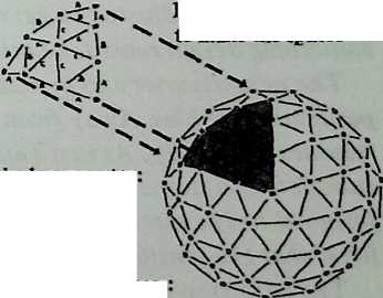
¶ Great Circles
A geodesic dome is sliced from one of the complex polyhedra we were learning to design in Chapter 5. It has a large number of triangular faces, all approximately but not quiteequilateral. The struts that bound them follow the paths of great circles, sometimes complete, more often interrupted. The cohesion of the whole, like that of a Tensegrity, is both compressive and tensile; it is helpful to imagine the tension system running along the outer surfaces of the struts, which are simultaneously loaded in compression.
As we saw in Chapter 1 (Diagram 1.1), tensile forces in post- and-beam construction run along the under edges of the beams, resisting central sag. In Tensegrities, on the contrary, tensile forces surround the system, hauling the vertices outward and so removing the need for posts. The first large geodesic structure (Robert W. Marks, The Dymaxion World of Buckminster Fuller, Carbondale: Southern Illinois University Press, 1960, figs. 0.19-0.21) retained separate tension members, running to every vertex from pegs jutting from neighboring vertices; since then it has been clear that at moderate frequencies the tensile cohesion inherent in the upper surface of the strut has ample mechanical advantage, and in most domes the tensile members are inextricable from the compressive, concealing from the casual eye the crucial importance of tension.
It is evident that the hub systems, as well as the struts themselves, must resist pulling forces as well as pushing forces. When heavily loaded, either by its own weight or by an imposed stress, a geodesic system will tend to pull apart at some of the hubs.
Again, make a model before proceeding further. Diagram 7.1 shows a simple 3v.icosa; connections are flexible; clearly the strength is derived from geometry, not joinery.
Experiment.
Try removing one strut.
Try removing one connector.
Note that at exactly twelve points, evenly distributed about the sphere, five triangles meet at a vertex. Elsewhere, the number that meet is always six.
Make an icosahedron (Diagram 7.2) with twelve more connectors and twenty struts of equal length. Note the five triangles meeting at each vertex. Observe the resemblance to the 3v icosa sphere.
Finally, observe the circle patterns. The five-way vertices are called pents (after the pentagons that surround them). From each pent center radiate portions of five great circles. Each has its center at the center of the system. Each sets off on a 360° circuit, of which it completes about 63.5° before bumping into another pent center (Diagram 7.3).
But if you follow the lead of any pentagon edge, you can trace a circuit clear around the sphere. This is a lesser circle; its center is not at the center of the system. They girdle the sphere in parallel pairs (Diagram 7.4), like the Tropic of Cancer and the Tropic of Capricorn.
It is natural to think of cutting the sphere along one of these lesser circles to get a tall ora shallow dome. Try it by unfastening connectors. Your first discovery will be that the dome does not sit quite flat: the struts in the lesser circles are almost, but not quite, coplanar. Obviously, the lengths of struts leading to the lesser circle could be adjusted to get a level truncation plane. That’s something design must take into account.
The next discovery to be made from a dome model is that the perimeter wobbles. Away from the perimeter, the structure resumes its rigidity. As in a Tensegrity, tensile circuits must be completed. A dome design is not completed until its lower edge is fastened to the earth. It is ultimately the inelasticity of the earth itself that the tensile network transmits through the structure.
The next step in investigating domes and great circles is to make a companion model based on the octahedron instead of the icosahedron. Diagram 7.5 gives data. Comparing the two models, we notice several things immediately.
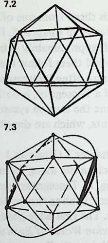
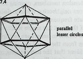
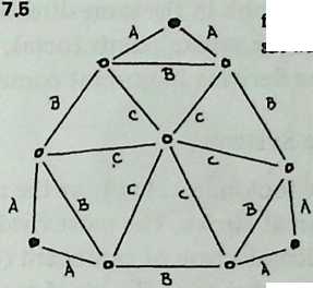
-
The octa uses fewer struts and connectors, and has fewer faces.
3v Icosa
3v Octa
edges 270 108 vertices 92 38 faces 180 72 -
The octa is much less smoothly spherical This derives from the fact that an octahedron is a poorer approximation to a sphere to begin with. Its sphericity can be improved by raising the frequency. A octa has a component inventory comparable to that of the icosa (300 edges, 102 vertices, 200 faces) and is comparably smooth in curvature.
-
Instead of the icosa’s twelve pents, we find six squares, corresponding to the six vertices of the parent octahedron.
-
Like the icosa’s great-circle arcs from pent center to pent center, the octa has great-circle arcs running from square center to square center. But instead of being intercepted at the next square center, each meets a partner at 180° and in effect continues straight through. Thus every octa, regardless of frequency, has three mutually perpendicular great circles outlined by its struts, making natural hemispherical truncation planes. (Icosas display hemispherical great circles at all even frequencies.[5])
-
Like the icosa, the octa also displays wobbly lesser circles. Truncation at other than hemispheric intervals will require adjusting strut lengths to make one of these lesser circles planar.
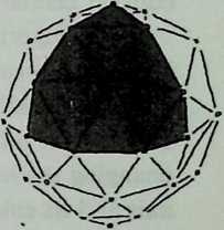
It is clear that certain characteristics of the parent polyhedron carry over into its geodesic derivates. The icosahedron has no vertex-to-vertex great circles, and neither has any of its geodesic subdivisions. The octahedron on the other hand has three, and so have its breakdowns. The icosahedron has twelve vertices where five triangles meet, the octahedron six vertices where four triangles meet; the same is true of their frequency subdivisions. (In either case, all other vertex points are hexagonal, by-products of the three-way grid.) Most important, an observer at the center of the system would look in the same directions to see the same pent points (icosa) or square points (octa), regardless of frequency. We shall later be deriving important consequences from this fact.
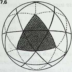
¶ Great-Circle Systems
We can now look more closely at the relationship between polyhedra and great circles. The most vivid look is prepared for by making an icosahedron of cardboard (twenty equilateral triangles, about 2 \sfrac{1}{2} inches to a side, glued together at the edges with contact cement).

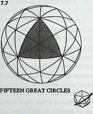
Press fingertips to a pair of opposite vertices and turn the icosahedron on the axis your fingers define. If you now imagine it spinning rapidly, you can see where the equator of spin would lie. If you next move the fingertips to a new pair of vertices without changing the icosahedron’s orientation in space, it acquires a new axis and its spin will trace a new equator, inclined to the first. If you keep this up till you have used all six pairs of opposite vertices, you will have six equators symmetrically intersecting one another. Diagram 7.6 shows all of them and shows how they symmetrically subdivide the faces of the spherical icosahedron. This is the family of the six great circles.
We next repeat this exercise, using mid-edge points for the poles of spin. There are fifteen pairs of opposite edges, and rotating the icosahedron between fingers pressed to the midpoint of any pair will describe an equator like the one in Diagram 7.3, cutting through two pairs of triangles and coinciding with two edges. By the time we have used all the axes of rotation we have located the fifteen great circles. Diagram 7.7 shows how they outline every icosahedral face, and also slice through every face three ways.
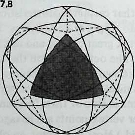
There is one more great-circle family, which we locate by using mid-face points for the poles of spin. (A triangle’s mid-face point is located by joining each vertex to the midpoint of the opposite side. It is two-thirds of the way down each altitude and is also called the triangle’s center of gravity.) The icosahedron has 10 pairs of opposite faces, and spinning it successively on an axis passing through each pair gives us the ten great circles. Diagram 7.8 shows how they are located. If we follow any one of them along its successive crossings of icosa triangle edges, we shall see that it repeatedly leaves the midpoint of an edge to cross the next edge at right angles.

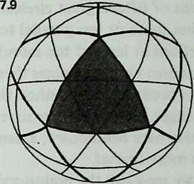
So the icosahedron has three families of symmetrically placed great circles, totaling , or .
We can now try some combinations. Start with the six great circles. Next outline the faces of the spherical icosa; we do this by using portions only of the fifteen great circles. Diagram 7.9 shows the result: a geodesic breakdown. If the vertices were joined by chords instead of arcs they would diagram a perfectly useful structure. They would be of two different lengths, and the longer ones would follow the six great circles. The shorter members, outlining icosa edges, define portions of interrupted great circles. The subdivisions tend to run in the same directions as the icosa edges, and we see at once why any emz-frequency subdivision of this general design will yield equators: they are the six great circles.
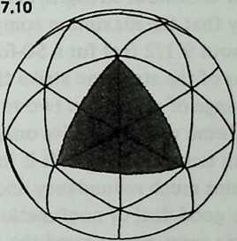
We now try something else. Commence with the fifteen great circles, and this time remove the portions that outline icosa edges, leaving everything else. This gives us (Diagram 7.10) another breakdown, this time with no complete great circles at all. (By adding four members, to complete two icosa edges, you could make an equator that coincided with any one of the fifteen great circles. The new members would cut four triangles in half.) This kind of breakdown, cutting perpendicularly across icosa edges that are no longer present, is called Class II. (The breakdown discussed first is Class I.)
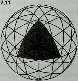
We may remember that the ten great circles also cut icosa edges perpendicularly, and try inserting them. Diagram 7.11 shows why this is unsatisfactory. It approximates a breakdown, but the triangles are of markedly different sizes, and some of them are excessively isosceles.
Still, we can understand why, in the pioneer days of geodesics, this sort of subdivision was the first to be explored: it promises access to the largest inventory of great circles, potentially twenty-five. Breakdowns of this general configuration were at first called regular, later triacon (after the rhombic triacontahedron, whose contours it suggests). It proceeds by joining each vertex of a tri-angular icosa face to the midpoint of the opposite edge (which gives portions of fifteen great circles) and running additional lines of subdivision more or less parallel to these (which with luck will pick up portions at least of ten more). In the finished artifact only this grid remains: the icosa edges themselves disappear. Later investigation produced the method that yields subdivisions parallel to triangle edges. Being an alternative to its predecessor it was called the alternate breakdown, a name that has stuck, though “Class I” is more formal.
In what we may call the prehistory of the art, there were no breakdown systems at all. Buckminster Fuller’s first experimental domes were simply sets of icosahedral great circles, made of short chordal members bolted together. All thirty-one great circles made a structure of enormous strength, and they intersected one another so frequently that the maximum component length was never excessive (about 9 1/2 feet for a 50-foot-diameter structure). Still, disadvantages of the structure strike the eye: component lengths vary over a range of more than two to one, and so does vertex population. Some vertices receive only four members; others are cluttered with ten and twelve.[6] It is intuitively obvious that such a system contains much redundancy and (putting the same thing differently) a good deal of nonfunctional weight.
Omitting six great circles eased the clutter somewhat; there were families of structures with twenty-five great circles. The next step, obvious in retrospect, was perhaps the most difficult to conceive: interrupting fifteen of the twenty-five great circles by removing members that outlined icosa faces (Diagram 7.10), and extending members that had terminated on an icosa edge to reach into the next triangle. All vertices were then sixes and fives, and strut-length variation was just under 2 to 1.
The system was how about to take its leave of what seems to us, decades later, a naive dependence on inherent great circles. (The name geodesic dome preserves the memory of that initial dependence.) It is obvious that more members can be introduced, parallel to the ones we have. This gives rise to the concept of frequency subdivision. It also permits the shorter component lengths we shall heed for very large structures. It is also obvious that by tinkering with the geometry we should be able to bring strut lengths closer to equivalence. The systems of geodesic breakdown commence at this point.
¶ Octahedral and Tetrahedral Great Circles
The octahedron too has three families of great circles, which the same experimental method will locate. The three vertex-to-vertex axes yield three great circles, which coincide precisely with the octahedron’s edges. Mid-edge to mid-edge axes yield six great circles, of which three appear on any single face, coinciding with its medians. The axes passing through opposite pairs of mid-faces yield four great circles, of which any face exhibits parts of three, joining the face’s midpoints. So the octahedron has great circles, of which any face is bounded and crisscrossed by 9.
If we design a geodesic sphere or dome by subdividing an octahedron, this set of thirteen comprises all the complete great circles we can possibly obtain. All others will be interrupted. Any Class I subdivision yields three, the ones bounding the octa edges. (Hence all Class I octa subdivisions have natural equators.) Any even-frequency Class I octa subdivision has these three and also four more (look back at Diagram 5.2). So all even-frequency Class I octa subdivisions contain seven complete great circles each. But as long as the lines of subdivision run parallel to the octa edges, there is no way to incorporate the remaining six great circles at all. Class II subdivision gives us access to these, but loses the other seven.
The tetrahedron, in this as in many other respects, is bafflingly economical. It has no opposite pairs of vertices. Each vertex is opposite a mid-face, and joining these unmatched pairs by axes we obtain four equators of spin, four great circles, of which any single face exhibits parts of three. Axes through pairs of midedge points yield another four great circles, of which each edge again exhibits parts of three, joining its mid-edge points. That is all.
An even-frequency Class I subdivision will display the first set, and if the frequency is divisible by 4 the second set will be present, as well. Class II subdivisions with frequencies divisible by 4 display the second set of great circles if they follow Method 1 (see Chapter 10) but none at all if they follow Method 3.
¶ Symmetry Systems
Symmetry is a measure of a system’s ability to absorb rearrangements that cannot be detected. A jigsaw puzzle has none; if you try to interchange two pieces, fit is destroyed. By contrast, square tiles in a square box can be permuted indefinitely without anyone’s noticing. An equilateral triangle which we are forbidden to tum over can be placed on the table three waysany vertex upward with no likelihood of these states’ being distinguished.
When we turn a polyhedron on an axis, as we did when we were eliciting the great-circle families in Chapter 7, it passes through a sequence of successive states that cannot be told apart. If the icosa axis runs vertex-to-vertex, a complete rotation brings five successive aspects to the fore, each indistinguishable from its predecessor. Each mid-edge axis yields two indistinguishable positions, and each mid-face axis three. So the three great-circle families correspond to three groups of rotational symmetry, and it is not surprising that we can discover symmetries in the inter- relationship of the great circles themselves. In fact, the icosahedron’s thirty-one great circles can be completely specified with the help of a small triangular module, shown in Diagram 8.1. Systematically rotated and reflected six times per spherical icosa face (thus, times per sphere) it reconstitutes the entire great-circle system. This little triangle thus contains all the information we need to subdivide a sphere with symmetrical great-circle systems. Any further subdivisions we may execute within the symmetry triangle will likewise be propagated throughout the system. The symmetry triangle is thus a kind of geodesic DNA molecule, and so long as we are concerned with spheres we may confine our interventions to its minute terrain, in confidence that the rest of the system will reproduce them exactly.
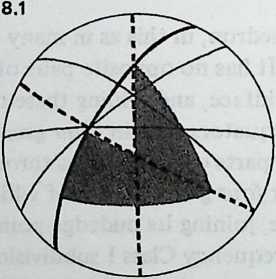
The octahedron has a corresponding symmetry triangle, which covers not but of its spherical area. Inspecting a spherical tetrahedron likewise, we discover a symmetry triangle that comprises of it. Since it can be shown that these three polyhedraicosahedron, octahedron, tetrahedron contain the entire available array of great-circle symmetry systems, there are no other cases we need to consider.
It is helpful to think of the polyhedron simply as a device to help us find systems of symmetry.
You are standing at the center of a polyhedral structure. You observe the repeating faces, the uniformly radiating edges, the equidistant vertices. These locate the reference points of omni-symmetry. A vertex, a face center, a mid-edge, comprises their minimum set. The little right-angled triangle so marked out the symmetry triangledefines all the polyhedron’s capacity for changes-that-do-not-make-any-difference. Its corners are the poles of symmetry, and if we could locate and specify them somewhere on a single polyhedral face, we should have control of the whole omnidirectional array. To see how this might be done, we shall imagine sightlines from the center of the system and find an economical way to specify them.
The great sphere of the sky, a man-made geodesic sphereit doesn’t matter which we think of: the sightlines are equivalent. The sky has one advantage: it frees us from error in locating the center. You are always at the center of the celestial sphere.
We can’t see the whole sphere, but it suffices to see the upper half of it. Imagine an unimpeded horizon, up from which arches the hemispherical bowl. One point on this bowl is perfectly unambiguous, the point directly overhead and equidistant from every point on the horizon. Call it .
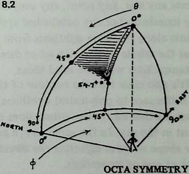
We can now designate any direction we choose with the aid of just two numbers. The first number is a compass direction: zero if we are facing north, an increasing number of degrees as we turn counterclockwise from north. The second number also specifies degrees: zero at the zenith, 90° at the horizon, other figures in between. Thus 0,45 designates a unique direction: north, and halfway from zenith to horizon. The comers of the octahedral symmetry triangle are at (see Diagram 8.2; the derivation of this last figure will be explained later).
Within the symmetry triangle we may specify in the same way additional points, each with its pair of numbers. We can choose them so that they locate whatever great circles we intend to use, and the vertex points for the geodesic breakdown we plan to employ. Each point designates a sight-line, and what we shall have specified is a cluster of sightlines which contains all the information we need to build a geodesic structure. The symmetry triangle and the cluster of points it contains would simply be reproduced, over and over, until the whole hemisphere was contained or the whole sphere, for that matter.
If you were standing at the center of a man-made geodesic hemisphere you would see the vertex points these sightlines designate, all joined by structural members in triangular arrays. With a little study you could locate the boundaries of an enclosing symmetry triangle and verify that it was the module of repetition.
¶ Envelope Contours
We are now about to derive advantage from the fact that we have directed our reference sightlines at the sky instead of at something more accessible like a planetarium ceiling. The advantage inheres in the fact that the sky has no definite distance. Celestial locations are nothing but a set of distance-less directions. Despite the three-dimensional ambience, two coordinates, not three, will suffice to locate any star, any point, any polyhedral vertex. Big or small, any icosahedral or any octahedral system disposes its reference points along the same sightlines from the center. We can therefore treat the whole system as a set of directions and invoke the distances later when we need them.
It’s also clear that the contour of the bounding surfaces makes no difference to polyhedral sightlines. The fact that some stars are much further away than others does not affect their relative placement in the sky. In the same way, a geodesic envelope may be of any shape without affecting the direction in which we sight to look at one of its vertices.
Provided the structural members were thin enough for their apparent width to provide no cues, it would be quite impossible for an observer at the center of a man-made structure to tell whether he was surrounded by a geodesic sphere or a geodesic egg. In the former case his eye’s distance from every vertex would be the same, in the latter case it would vary, but, given a structure so refined its members looked like ruled lines, these two cases would display exactly the same angular symmetries.
In separating distance from direction, we have taken a step of great potential usefulness. First, we know better what we shall be about when we execute a geodesic breakdown. The breakdown will be a little cluster of sightlines, a local symmetry occupying one symmetry zone of the great polyhedral symmetry, and repeated as often as the structure we envisage may require. The envelope of that structure will intercept our system of directions at various points. These are the points that will be joined by struts, and the length of the struts will depend wholly on the size and contour of the dome we want to make. Specify these, and from a table of angular sightlines it is simple to calculate the distances.
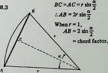
It is evident from Diagram 8.3 that if is the angle between the sightlines that lead to two vertices, and is the distance of each vertex from the center (the uniform radius, in the case of a spherical system), then the strut length between the points is multiplied by , twice the sine of half the angle. Twice the sine of half the angle is called a chord factor, because the strut is a chord and we have here one of two useful factors of that chord, the other being the radius. Geodesic designers have worked with chord factors ever since Fuller introduced the concept in the early 1950s. Tables of chord factors, containing as they do the essential design information for spherical systems, were for many years guarded like military secrets. As late as 1966, some icosa figures from Popular Science Monthly were all anyone outside the circle of Fuller licensees had to go on. Now, thanks largely to Lloyd Kahn’s Domebook 1 (Los Gatos, Ca., Pacific Domes: 1970) (Khan 1970) and Domebook 2 (Bolinas, Ca., Pacific Domes: 1971) (Khan 1971) chord factors for at least small-to-medium structures are fairly accessible.
But concentration on chord factorsthe information a constructor ultimately wantshas concealed the great usefulness of the angles from which they are derived. If we know the chord factors for a sphere of a given breakdown and frequency, we can proceed to duplicate it in any practical size. But if we know the sighting angles, we are no longer restricted to spheres. By allowing the radius to vary harmoniously from point to point, we can derive chord factors for a dome of any useful shape. There is no need whatever for geodesic structures to be spherical.
What we are after, therefore, is a local cluster of symmetrically disposed points, their symmetries expressed as angles between sightlines from a common center. Once we have our cluster of points, which will be denser for higher-frequency breakdowns, and have made a table with sighting angles for each, we shall need only a procedure for determining the chordal distances from any point to its neighbors, whether they are at the same distance outward or not, and we shall be equipped to design geodesic structures of any shape we please.
¶ The Spherical-Coordinate System
We have learned that two anglescall them and will specify a direction, and two angles , together with a distance will specify a unique point. These are the elements of the spherical- coordinate system, which is less well known than it might be. Most problems of geodesic mathematics can be solved with its aid with straightforward ease.
The coordinate resembles a meridian of longitude. All points with the same lie on the same great circle, which passes through the zenith . It is convenient to incorporate the reference meridian, , into our calculations whenever we can. The first coordinate of all points situated on it will be 0. The coordinate resembles a specification of latitude, except that it is measured down the circle from at the zenith, instead of upward from the equator. (In the spherical-coordinate system, the equator is at .) All points whose second coordinate is lie on the equatorial great circle. With the exception of these, all points with the same lie on the same lesser circle and specify a plane along which the dome can be truncated so it will sit flat.
The coordinate, measured not in degrees but in units of length from the center, tells us how far out a point is to be found. If the points are on the surface of a sphere, like the vertices of a spherical geodesic structure, we can let and virtually disregard it. The angles and tell us all we need to know. If the envelope of the system is other than spherical, then varying values of will have to be taken into account.
Now for the usefulness of understanding this system. If we know the coordinates and of two points, then we can find the distance between them by inserting these values into an equation which a pocket calculator can readily subdue. The result, , will be in the unit used for and , and if either of these distancesor both in the case of a sphereis made equal to 1, the result will be a chord factor.
For the spherical case, when, this becomes
For a first example, check back to the octahedron we discussed in Chapter 5 (Diagram 5.4). Diagram 9.1, with the same lettering, shows how this looks in spherical coordinates. , are the corners of one octahedral face. Their coordinates are . The edge midpoints have the coordinates . Because the system is symmetrical we need only two distances: a vertex to a midpoint, and a midpoint to a midpoint. and will suffice. Because the system is spherical we use Equation 9.2. The sines and cosines we shall need are as follows:
| cosine | sine | |
| 0^ | 0 | 1 |
| 45^ | 0.70710678 | 0.70710678 |
| 90^ | 1 | 0 |
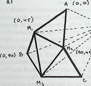
Inserting these values into Equation 9.2, we get for (coordinates and ):
d=V2- 2(0.70710678 + 0)
=V2 - 1.41421356 =V0.58578644 = 0.765367
And for (coordinates 0,45 and-90,45) we get
d=V2- 2(0.5 + 0)
= V1
= 1.0
These answers agree exactly with those we obtained by other means in Chapters 5 (Diagram 5.5). And since they are multiples of when , they are identical with the chord factors introduced in Chapter 8.
True, the purely geometrical argument in Chapter 5 yielded the chord factors with less manipulation and in less time. But that was a case. Raise the frequency, and the geometrical method soon becomes too cumbersome to stay in the running. (Desert the spherical contour, and it becomes nearly impossible.) Moreover, each result yields data for its successor, and an early error invalidates subsequent work. The 0,0 method, on the other hand, permits a standardized procedure. All chord factors are found by exactly the same routine, and all are found independently; errors are isolated, and do not affect other computations. And a good pocket calculator, which can quickly change angles into their sines and cosines and has no more trouble with roots than with 2 4-2, permits us to run through the chord-factor equation for each pair of points in less than a minute, even when coordinates are cumbersome. (Suitably programmed, the ultra-sophisticated HP-65 will do the computing in four seconds per case.)
While we have in front of us data for a simple case, we may as well experiment with Equation 9.1. What if we wanted to make this simple dome elliptical? Let us specify a beehive orientation (Diagram 9.2) 11/2 times as high as it is wide. A hemisphere of 20-foot diameter would thus be stretched to give not 10 feet of headroom but 15.
We see at once that the radius varies with . At the zenith , . At the floorline (0 = 90°), . At the octa mid-edge (0 = 45°), the reader may take it on trust that . (We shall learn later how to calculate for any value of 0 in ellipses of any proportions.) These are the only values of 0 we have to deal with, so we make a table:
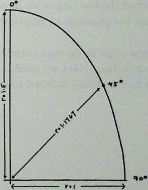 9.2
9.2
e r
0° 1.5
45° 1.1767
90° 1.0
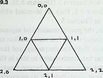
Since continues to vary beyond the confines of the octa symmetry triangle, we should identify the various vertices in a face triangle (Diagram 9.3 shows a useful notation) and decide how many different chord lengths we must deal with. 20/21 and 21/22, where , will be just the same as before. But since 0,0 and 1,0 have special values for r, we shall need 10/11,00/10, 10/20, and 10/21. But the system retains mirror symmetry (1,0 has the same 0 as 1,1), so 00/11 will equal 00/10, 10/20 will equal 11/22, and 11/21 will equal 10/21. So we need four new chord factors, which we obtain by putting the proper values of 0, 9, and into Equation 9.1. Thus 10/21 is given by:
The reader may verify that is , is , and is .
A model built to these specifications would be far from smooththe frequency is simply too low to record nuances of elliptical curvaturebut the few points we have are correctly located, and it is clear that the principle of elliptical domes presents no real difficulties.
So we know what to do with coordinates of breakdown vertices on a polyhedron face. Next we need to know which polyhedron to choose, and how to break it down to obtain the coordinates themselves.
¶ Breakdown Systems
We start with the breakdown systems, because they provide some of the criteria for choosing a polyhedron. All systems start with a triangular polyhedron face and subdivide it with a three-way grid. We then push all the vertices of this grid outward till they are a common distance from the center (for spheres) or a harmoniously varying distance (for elliptical and other contours). When we have done this, some of the lines of subdivision will follow great circles inherent in the polyhedron’s symmetry. We want the ones that don’t do this to trace at least partial great circles, interrupted by the edges of polyhedron faces. And we want to maintain a reason- ably symmetrical spacing, so that the little triangles we have created will be nearly equilateral. We shall commence our thinking about all this by examining the first of the two basic ways to orient the grid.
¶ Class I (Alternate)
The grid lines run roughly parallel to the edges of the polyhedron face.
We want to specify the crossing points, and there are a number of different techniques, all of which yield slightly different strut lengths. All are correct, in the sense that they generate three-way grids with sphere vertices equidistant from the system center. Some are of historical interest chiefly. Still, there are choices to be made, and particularly at low frequencies we may be guided between two principal methods by a rather simple choice: similarity of triangle size, or similarity of triangle shape.
A worked example will clarify this. To keep figures few and simple we shall use the octahedron and compare two methods of making a Class I breakdown.
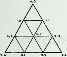
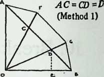
Diagrams 10.1 and 10.2 show Method 1. It amounts to drawing a triangle face on flat paper, dividing its edges equally, then projecting the division points outward to obtain equal radii. It is clear from Diagram 10.2 that although the divisions A C, CD, DB are equal, the chords AF, FG, GB are not (the end chords are shorter than the central one). The sighting angles from the center to the chord ends will differ likewise, so the coordinates will be unevenly spaced. Diagram 10.2 shows a construction for obtaining them. As for the triangle’s center point, we have learned that it is 54.7356° inward from each vertex (coordinates 45, 54.7356). Equation 9.2 will give us chord factors as shown.
0 |
||||
| 0,0 | 0 | 0 | 0,0/1,0 | 0.459506 |
| 1.0 | 0 | 26.5650512 | 1,0/2,0 | 0.632456 |
| 1.1 | 90 | 26.5650512 | 1.0/1,1 | 0.632456 |
| 2,0 | 0 | 63.4349488 | 2,0/2,! | 0.671421 |
| 2.1 | 45 | 54.7356103 |
Method 2[7] simply spaces the coordinates equally down th octa edge (30°, 60°, 90°), making all edge struts equal. The triangle’s center is located as before, and we proceed (Diagram 10.3) to obtain chord factors.
We should now look at models, and folding paper is an easy way to make them. Diagram 10.4 and Diagram 10.5 show patterns for one octa face computed by each method. Four of either, cut out and creased, can be taped together to make a hemispherical dome. By simply looking at the diagrams we can see a marked difference. When we have equal chord factors along the octa edge (Method 2), the small triangles vary less in size, but vary more in shape. Disregarding for the moment the comer triangles/1, which are always a special case, we notice that the rest of the octa face is shared by three each of two quite noticeably isosceles triangles, and C. But when we vary the edge chord factors (Method 1) the corner triangles stay virtually the same shape as before, while the rest of the octa face divides itself into 6 identical triangles , which come much closer to being equilateral than either or Cin the other diagram.
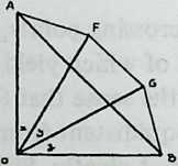
In short, by letting the triangle sizes vary more we can keep their shapes more nearly constant.[8] This seems structurally as well as aesthetically preferable. The more nearly equilateral a triangle, the more nearly equilibrated should be its resistance to pushes and pulls from various directions. The price, a more marked variation in strut length, has been carried to extremes by the present example. It is less marked at high frequencies than at low, and less for the icosa than for the octa. A octahedron is about the worst possible case.
0,0/1,0 0.517638
1,0/1,1 0.707107
2,0/2,1 0.650115
0 |
||
|---|---|---|
| 0,0 | 0 | 0 |
| 1.0 | 0 | 30 |
| 1,1 | 90 | 30 |
| 2,0 | 0 | 60 |
| 2,1 | 45 | 54.7356103 |
method 2 coordinates
Since Method 1 appears to be the Class I breakdown of choice, we shall stick to it for the rest of the book.
A word about triangle shapes in general. Though the norm is an equilateral triangle, it is clear that if the little triangles were really equilateral we should have neither dome nor sphere but flat grid-work. It is their departure from equilaterality that provides the curvature, as we can see by considering the sum of the angles around a single vertex. Around the central vertex in Diagram 10.5, the apices of the triangles total 6 X 56.2°, or 337.2°. This is nearly 23° short of the 360° that would lie flat; the shortage is called the spherical excess of the vertex. Descartes showed long ago that the spherical excess of all the vertices in any polyhedron must always total 720°. Since there are 38 vertices in a octa sphere, we should find an average spherical excess of nearly 19° at each of them. The vertex we have just looked at has more spherical excess than the average, and so have seven others like it; they are contributing to a deficit incurred at the vertices where four octa faces meet, and where 4 X 86.9° = 347.6° gives a spherical excess of barely more than 12°.
It is at these latter verticesthe octa’s six squares, the icosa’s twelve pentagonsthat we are most likely to find deficient spherical excess, in other words a tendency to flatness. Flattish vertices are more likely to pop in under load, one reason it is desirable to keep spherical excess more or less evenly distributed (and triangles more or less equilateral).
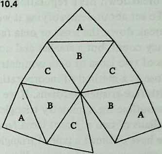
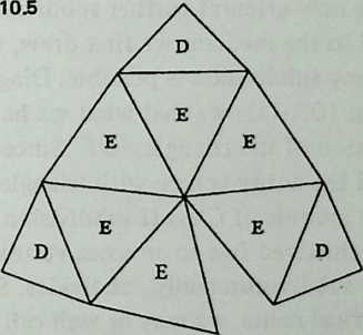
¶ Class II (Triacon)
The grid lines run roughly perpendicular to the edges of the polyhedron face.
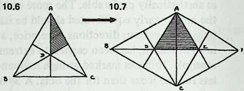
This breakdown has a reputation for being difficult to under- stand. To set about demystifying it we may note that it does not really break down the icosa or octa face from which it derives its frequency count, but a smaller and nonequilateral triangle which consists of two icosa or octa symmetry triangles back to back.
It arose as a method of incorporating the great circles that coincide with face-triangle medians. If we draw the three medians of a face we outline the symmetry triangles (Diagram 10.6). If we draw the medians of two adjacent icosa faces (Diagram 10.7) we find that we have outlined a pair of triangles, and , each com- prising two symmetry triangles. If we continue in this way to sub- divide the entire icosa (Diagram 10.8) and then eliminate the icosa edges themselves, we have a Class II breakdown, made up entirely of triangles like ADE.
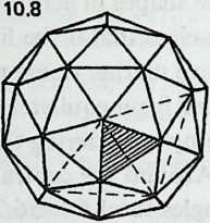
If we now attempt further subdivision of the icosa face by lines parallel to the medians we first drew, we discover that only even-frequency subdivision is possible. Diagram 10.9 shows 4j>, and Diagram 10.10 shows that what we have really achieved is a subdivision of the triangle ADE. Since in Diagram 10.8 we had covered the entire sphere with triangles like , such a triangle is the real module of Class II subdivision. There are sixty such triangles, clustered five to an icosa vertex, and they are what the Class II subdivision really subdivides. Since they seem to have no geometrical name, we may as well call them Class II triangles. (The diamond ADEC, made up of two of them, is one face of a spherical rhombic triacontahedron, hence the nickname triacon for this breakdown.)
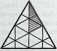
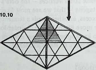
Once more there are several methods, of which we shall find uses for two.
Method 1 in effect divides the diamond median (= icosa or octa edge) exactly as in Class I, Method 1, to yield equal parts on flat paper but unequal chords when the vertices are pushed out to make spherical radii equal. We then concentrate on one half of the diamond, the Class II triangle, and run perpendiculars from the median outward to the sides. The triangle’s bottom edge is now subdivided the way its median was, and lines join these edgepoints to complete the grid.
The result is a strikingly symmetrical breakdown, and a little more economical of components than Class I, but not much. Its symmetry module is the icosa or octa symmetry trianglethat is, half a Class II triangle. (At first glance one might expect the module to be smaller, but the Class II triangle isn’t equilateral.)
The other Class II system we shall find useful is called Method 3 in Clinton’s “Geodesic Math” article, where we find it credited to Duncan Stuart. It is one of the most ingenious achievements in the short history of geodesics, permitting as it does an absolute minimum member-length inventory - 4 for 4p, 12 for 1, and so on. We pay for its economy by accepting less symmetrical breakdown triangles. Diagram 10.11 shows the principle; the horizontal members cross the Class II triangle’s median at equally spaced intervals, and the bottom edge-point divisions are directly below the corres- ponding side-edge divisions (broken lines are at 90° angles with bottom edge). It now turns out (Diagram 10.12) that each side-edge division will propagate itself by zigzagging all the way down the main triangle, and each horizontal division will recur as a set of parallel reflections. The figure shows members of eight lengths for 8p. The chord factors show the asymmetries we accept; all members shorten as we move downward and outward.
Still, the saving in different member lengths is remarkable. This method requires 12 lengths for 12i>. A Class II Method 1 of the same frequency requires thirty-two, and a Class I Method 1 requires forty. It is not surprising that most of the largest geodesic structures hitherto have used Class II Method 3 components.
Of course we realize these savings only with spheres. Once the member length commences to vary with the radius, as in the case of ellipsoids, Method 3 loses all advantage over Method 1. For small Class II spheres, Method 1 gives visibly smoother arcs. But if you need to design a very large geodesic sphere and have any concern at all for economy of fabrication, Class II Method 3 is the place to start.
l.a, a, a, a.
equal divisions of median.
2. Solid lines:
Horizontals locate
edge points.
3. Dashed lines:
perpendiculars
locate mid- and
bottom points.
4. Dotted lines:
final grid.
10.11
METHOD 3 BREAKDOWN OF
CLASS II TRIANGLE, 8p.
10,12
SYMMETRIES
(LEFT HALF)
CHORD FACTORS
0.170287
0.199457
0.167003
0.195678
0.161026
0.184914
0.153316
0.168672
Values decrease
toward bottom
left (and, by
symmetry, toward
bottom right).
¶ Which Class?
We may now review the characteristics we have noted in passing.
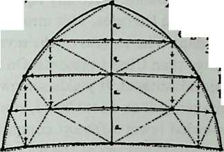
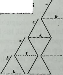
Class I keeps component variations within narrower bounds, but does so at the cost of employing a larger inventory of different strut lengths (how much larger depends on the frequency, and increases rapidly). It permits odd as well as even frequencies, a greater advantage for simple systems than for complex. (Dropping from 4p to 3v permits notable economy; the saving of 1 Ip over 12p is quite unimportant.) Class I icosahedra have uninterrupted equators at all even frequencies, and at all frequencies numerous undulant lesser circles which we can straighten out by a method to be described later and use as truncation planes.
Class II yields even frequencies only. Used with the icosahedron (though not the octahedron or tetrahedron) it introduces some truncation problems, since any equator breaks through some of the subdividing triangles. This means figuring special members to close the gaps. The lengths of the several components vary over a wider range than Class I presents. On the other hand, Class II has economic advantages. It yields somewhat larger triangles for the same frequency than does Class I, somewhat fewer components, and somewhat fewer different components. In Method 3, as we have seen, the shrinkage of the list of different components can be spectacular. And we shall see in Chapter 16 its special advantages for diamond-pattern and space-frame applications.
¶ Which Frequency?
The smaller the polyhedron face we are subdividing, the lower the frequency we shall need for acceptable sphericity. And the larger the structure we intend to build, the higher the frequency we shall need, to keep component lengths reasonably short. High frequencies not only use a great many struts, they use a great many different strut lengths, a fact that is less apparent to the eye when the high frequency subdivides an icosa face than when we are dealing with an octa or, worse still, a tetra.
In general, to minimize component inventory, we use the lowest frequency we can. How long a component we can tolerate is a function of its slenderness ratio (length divided by diameter). Fuller has suggested 24/1 as a slenderness ratio for wood, 30/1 for metal or prestressed concrete.
Finally, very high frequencies bring each vertex so near to flatness as to be dangerous unless virtual thickness is imparted to the shell by trussing (see Chapter 16). “Very high,” for the icosa, means anything over 1 with careful workmanship, or over, say, when tolerances are less than exacting.
¶ Choosing a Polyhedron
If our requirements are sufficiently modest, we need not start from a polyhedron at all. Standing at the center of the system we propose to design, we can surround ourselves with as many points as we like, obtained by writing coordinates by hunch, or even at random. We can join each point to its two nearest neighbors to obtain a triangulated network, and use Equation 9.2 to calculate the lengths of these connections. This gives us a table of chord factors. If we then choose a radius and let the chord factors determine the lengths of members, we can build a spherical environment which meets two important criteria. (1) It is spherical; every vertex point is at the same distance from the center. This fact is guaranteed by Equation 9.2, which treats and as spherical coordinates. (2) It is omnitriangulated, hence self-sustaining. We ensured this by our method of joining the points.
But it has grave deficiencies. (1) It is unlikely, except by chance, to possess any symmetries whatever, save that of the spherical envelope (a constant radius). This means that every single member length is probably unique, which is wildly inefficient. It also means that numerous short members are quite likely to be clustered in zones where they make no structural sense, and that elsewhere long unassisted spans are likely to bound large triangular openings. It means that if we want a dome instead of a sphere, no truncation plane exists, nor any logical place to go about inserting one. And it means that the structure looks as unpleasingly random as the design process was.
Moreover (2), it is very unlikely indeed that any sequence of vertices will be aligned along a great circle. Any two of them will be, because an equator can be made to pass through any two points on a globe. But that is not what we want to achieve. The geodesic dome, as we have seen, is supported by tension, and the tension networks are most economical when their strands run for considerable distances without changing direction. This means aligning sequences of vertices along great-circle arcs.
Hence the polyhedra, which we described in Chapter 8 as devices for finding symmetry systems.
There are only three such systems to be found: tetrahedral, octahedral, icosahedral. All other regular or semi-regular polyhedra present variations on these themes; thus the icosidodecahedron we encountered in Chapter 3 has icosahedral symmetry, and the cuboctahedron has octahedral. It is possible to execute a geodesic breakdown on any polyhedron, by triangulating its non-triangular faces before commencing, and a few polyhedra have special advantages. Thus A. J. Pugh has pointed out that since truncated octahedra cluster naturally, they make a natural starting point for domical clusters (Polyhedra, University of California Press, 1976). To isolate first principles, though, we shall concentrate on the three prime symmetry systems, tetrahedral, octahedral, icosahedra.
We commence by setting the tetrahedron aside, for use; only in a few very special situations we shall look at much later. Its overwhelming disadvantage is inefficiency. Having only four face triangles, it uses up so much of the sphere’s surface before repeating anything that to obtain an average chord factor of about 0.33 we must go all the way to subdivision (Class I). We then confront twenty different member lengths, varying over a range of . (By contrast, a icosa yields a slightly tighter meshaverage chord factor about 0.30 using only six different lengths which vary over a range of .) A Class II attack on the tetrahedron gives more attractive results and underlies most of its usefulness. It remains a special-case polyhedron merely.
For most purposes, then, we have the icosahedron and the octahedron to choose from.
Useful characteristics of the octahedron include:
-
a natural equator at all frequencies;
-
vertical slicing line at all frequencies, permitting half a dome to be joined to a rectangular structure;
-
simple generation of non-spherical contours;
-
provision for square openings: either one at the zenith or, by a simple rotation, three surrounding the zenith partway down;
-
relatively simple computations.
Useful characteristics of the icosahedron include:
-
lower frequency for comparable average chord factor (a icosa yields sphere subdivisions comparable to a octa);
-
angles uniformly averaged among nearly equilateral triangles (octa has right-angled triangles at its principal vertices);
-
less variation in the lengths of members for comparable average chord factor ( for icosa, for octa);
-
curvature more uniformly distributed (principal octa vertices are nearly flat; hence they are potential weak areas);
-
generally superior appearance.
Some of the icosa’s advantages disappear once we contemplate non-spherical contours. Since member lengths of elliptical or similar structures must vary continuously from the 0° zenith down to a 90° equator, the icosa loses most of the economy it derives from its generally lower frequency of subdivision. In addition, it requires us to subdivide two different triangles differently en route to the equator, while the octa comprehends this span in a single triangular face.
A minor disadvantage of icosaslack of a natural equator disappears at even frequencies, though only with Class I breakdowns, The octa can always be rotated to yield an equator, whether the subdivision is Class I or Class II.
As for the relative ease of computation afforded by the octahedron, this advantage is peripheral; computations, however troublesome, need only be performed once.
There seems to be no doubt that a wooden dome is easier to build from octahedral geometries; plywood panels, for instance, fit more easily at square than at pentagonal apices.
In Shelter (Bolinas, Ca., Shelter Publications: 1973) Bill Woods of Dyna Domes, whose user-built wooden structures use octahedral geometries and are reportedly trouble-free, is quoted as saying flatly that the icosahedron is “no good.” No reasons are given, but Woods presumably had in mind the octa’s adaptability to hammer-and-nail technology. Doors and windows, for instance, are easier to fit when squares, not pentagons, are available at the principal vertices.
¶ Other Criteria
We shall see in Chapter 14 that rotating an octahedron until the center of a face is uppermost places three square windows in symmetrical array around the zenith and about 50° down from it. Should we want this trio of skylights, only the octahedron will provide it, and only in a Class I breakdown.
Similarly, the Class II tetrahedron (Method 1), truncated on one of the great circles it makes available, affords at ground level four pairs of large, virtually square openings, each with a single diagonal brace, removal of which leaves a natural door (try an model). The tetrahedron’s drawbacks, notably its extreme variation in member length, might well be worth coping with should we want a structure with large doors in pairs at the four compass points.
As these examples indicate, some of the inherent difficulties of designing useful geodesic structures can be minimized by choosing the right polyhedron and turning it right way up. Truncation planes will often seem uneven, but in Chapter 14 we shall learn how easy it is to deal with that.
So there may well be practical reasons, deriving from a structure’s intended use, for selecting one polyhedron rather than another.
Or there may be aesthetic reasons. A geodesic framing system is normally visible, and we should give some thought to what it looks like. Near-equality of member lengths makes icosahedral systems especially graceful, and functions of the celebrated Golden Section pervade the proportions of the icosa itself and no doubt help account for its visual appeal. At the other extreme, a designer in quest of bold effects might do worse than investigate the Class II Method 3 tetra, a system of elongated diamonds with incised dihedral angles (again, try an model).
¶ Using the Tables
We now come to the actual coordinates and their use. Though a glance at the tables in Chapters 18–23 may suggest otherwise, the process by which they are obtained is almost ridiculously simple. Each pair is generated from a set of 3 integers whose sum is always the frequency of the breakdown, and for the octahedron, especially, the process of generation is so simple we seem closer to numerology than to engineering design. The following paragraphs explain how it is done for the reader who may some day want coordinates for some special frequency. The reader who simply wants to use the tables provided may skip to the next section of this chapter.
Diagram 12.1 shows how we get our sets of three integers. A diagram of one subdivided face is first numbered in the orderly fashion shown in the first drawing; this gives us the first integer of each vertex. The pattern is then rotated clockwise to obtain the second integer, and clockwise again to obtain the third.
Each vertex has now a unique three-integer label, and if we have made no mistakes, the sum of the integers at any vertex will always equal the frequency. Call these integers .
Now for the octahedron,
For the icosahedron, we obtain in exactly the same way, but before using the equations we convert into , as follows:
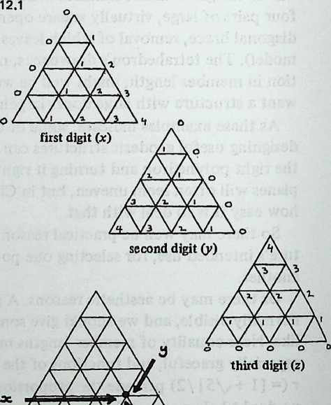
Here is the famous Golden Proportion, , or , or (this last form is the handiest to enter on the calculator). The icosa coordinates are:
For the tetrahedron, we convert into , as follows:
The tetra coordinates are:
This system gives us Method 1 coordinates. For Class II Method 3 (inferior symmetry, but maximum component economy) we require another system, which is explained in Appendix 3.
Inspection of the octa and tetra equations discloses the useful fact that all coordinates for these polyhedra are either rational fractions or the roots of rational fractions. Thus in an octa has the coordinates
Both values are given in the tables, but the former is quicker to enter on the calculator.
We shall now see how to use coordinates to design a geodesic structure.
¶ Planning the Work: Class I
Sketch an equilateral triangle (Diagram 12.2), subdivide the edges into parts for frequency, and join the points of subdivision with a three-way grid.
Now start with the top vertex and number all the crossing points, as shown. For frequency the last point on the bottom row will be . Every point now has a two-digit marker.
Now draw the three medians of the face triangle (vertex to mid-point of opposite side: the broken lines in Diagram 12.2). You have outlined six right-angled triangles, each of which contains the whole symmetry system of the polyhedron. Concentrate on the top left one, which we’ll call “the” symmetry triangle. If the structure we are planning is spherical, we need chord factors only for the breakdown edges that lie partly or wholly inside the symmetry triangle. For the example shown, this means only the twelve edges drawn with heavy lines: twelve out of sixty-three. For a sphere the only coordinates we need are the endpoints of those twelve edges: a total of ten coordinates. The rest of the system repeats symmetrically; thus corresponds to : six occurrences of the one length. Anything that cuts an edge of the symmetry triangle occurs only three times per face: thus, is repeated at .
All this is true of spheres. If we plan something elliptical we need more lengths, because the radius changes constantly as we move down from the zenith , and the top half of a face won’t duplicate the bottom half. We need coordinates as far down as , where the bend of the elliptical contour reverses itself. An octa or tetra face goes down that far; an icosa face doesn’t, and the icosa tables provide for a second face, drawn under the first and numbered as shown in Diagram 12.3. (For more details see Chapter 13.) Because of the steadily altering radii the symmetry triangles no longer contain all the different lengths, but we still have left- and right-hand mirror symmetry to cut down our work.
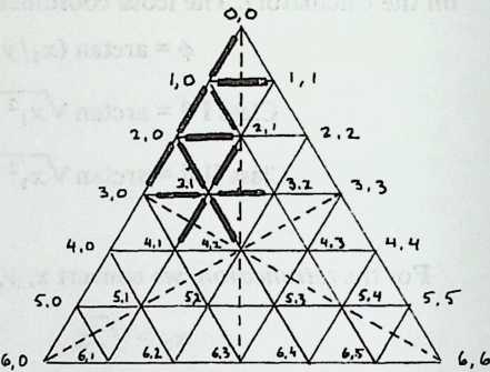
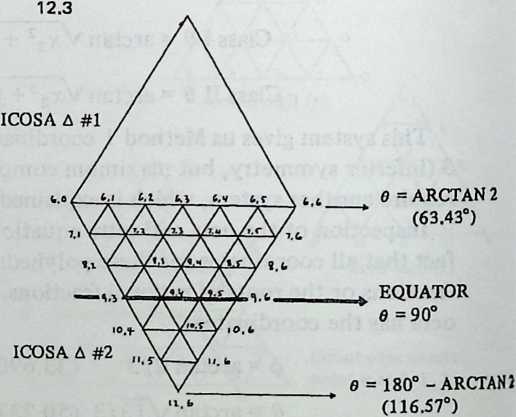
We now make a list of the coordinates we actually require. To keep the example simple, we’ll stick to the sphere.
Each face has actually six symmetry triangles, and we’d get the same chord factors whichever we investigated. But we use the top left one because the numbers to be manipulated are handier if we stay to the left, where many values are zero, and toward the top, where occurs and values are smallest. For a sphere the worksheet would look like this:
| ,0/1,0 | |||||
| ,0/1,1 | ,0 | ||||
| ,0/2,0 | ,0 | ||||
| ,0/2,1 | ,1 | ||||
| ,0/2,1 | chord | coordinates | ,0 | ||
| ,0/3,0 | factors | required | ,1 | ||
| ,0/3,1 | required | ,0 | |||
| ,1/3,1 | ,1 | ||||
| ,0/3,1 | ,2 | ||||
| ,1/3,2 | ,1 | ||||
| ,1/4,1 | ,2 | ||||
| ,1 /4,2 J |
Now we know which coordinates to extract from the table. Assume we want an icosahedral dome. We turn to “Icosahedron Class I Coordinates: Frequencies 6,3” (Chapter 20). Going down the “” column to the vertices we have just listed, we copy the coordinates as we find them. The list looks like this:
| ,0 | ||
| ,0 | ||
| ,1 | ||
| ,0 | ||
| ,1 | ||
| ,0 | ||
| ,1 |
27.2237351
3,2 49.6138225
4,1 16.0353713
4,2 36
16.0353713
39.1034177
37.3773682
Now we are ready for chord factors. Since our structure is to be spherical we use Equation 9.2 and insert pairs of values from this table. Thus for the distance of we use 0 for the values of and for . The chord factor turns out to be . The reader should now practice with the calculator and the equation until he gets the following results. Once your routine is debugged you can work with great confidence.
| 0,0/1,0 | 0.162567 | 2,0/3,1 | 0.198013 |
| 1,0/1,1 | 0.190477 | 2,1/3,1 | 0.205908 |
| 1,0/2,0 | 0.187383 | 3,0/3,1 | 0.205908 |
| 1,0/2,1 | 0.181908 | 3,1/3,2 | 0.215354 |
| 2,0/2,1 | 0.202820 | 3,1/4,1 | 0.215354 |
| 2,0/3,0 | 0.202820 | 3,1/4,2 | 0.216628 |
We see that we have more symmetries than we had been led to expect: there are three identical pairs, hence only nine different component lengths overall. With experience such duplications can be anticipated. But it is always safer to invest a couple of minutes figuring a superfluous value or two than to waste time and building materials on a false assumption.
A way of checking the work is to list the coordinates inside a different symmetry triangle entirely and calculate the values for these. Though we are working with completely different numbers, the chord factors should be identical.
Note that the longest members radiate from the point where the symmetry triangles meet, and the shortest from the comers of the face triangle. This is generally true of geodesic spheres, and gives us a quick test for improbable results. These two lengths are the extremes, and the rest should fall smoothly between them.
¶ Accuracy
We have given six-figure chord factors, and it is interesting to see what sort of accuracy this would yield in practice. We might envisage a hemispherical dome 100 feet in diameter (50-foot radius). This would entail strut lengths of the order of 10 feet, bigger than anyone is likely to go with 6v. The chord factor nearest the mean value is , and multiplying this by 50 feet we obtain a strut length for these particular members of 118.80780 inches. If we change the chord factor by +1 in the sixth place, we get 118.8084 inches, an error of 6 ten-thousandths of an inch. That is as much trouble as we are likely to get into by not using seven-place chord factors. Our coordinate tables are given to seven places (various rounding-off errors make the eighth place probable but not certain), so six places seems far enough to take chord factors.
¶ Class II
The design of a Class II structure goes in the same way, with a few variations. The triangle we draw and subdivide is not the polyhedron face but its Class II triangle, as shown in Diagram 10.10. It straddles the edge between two polyhedron faces, and its bottom edge joins their centroids. For -frequency division of the polyhedron, we make subdivision of its Class II triangle, and our module of symmetry is the entire left-hand half of this triangle. Diagram 12.4 shows the idea. For a Class II subdivision of the icosa face, we make a subdivision of its Class II triangle. Chord factors for the left half of this are duplicated in the right half, and the entire Class II triangle is duplicated by mirror symetry below itself, bringing us to the end of an icosa edge, which we find we have thus divided into 6. So much for Class II spheres.
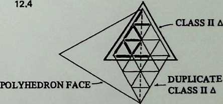
For the ellipse things are a little more complicated. To get down to the equator we need five symmetry triangles, as shown in Diagram 12.5 for an example. Note carefully how the numbering is done; the sequence 0,0; 1,0; 2,0; and so on proceeds down the left-hand edge, and such sequences as 4,0; 4,1; 4,2 follow the upward-slanting lines.
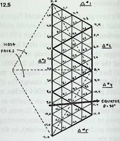
The equator always passes through the midpoint of the edge the two bottom Class II triangles share (10,2 in the example) and passes a little below the edge point at the left, a little above the edge point at the right. A glance at the icosa Class II Method 1 table confirms this; 1,0 has a 6 of 90, but the corresponding values for 9,0 and 11,4 are 88.95519820 and 91.04480176. So an equatorial cutoff just misses alternate vertices;
In Chapter 10 Class II Method 3 was presented as a system for maximizing the economy of different component lengths, at the cost of a slight loss in triangle regularity. Since this virtue applies only to spheres, the designer will be asking of this method none but spherical chord factors. So a complete set of these is provided in Chapter 23. They are ready for use without reference to the coordinates, which are presented only for their usefulness in two contingencies: the insertion of truncation planes (Chapter 14) and the design of space-frame structures (Chapter 16).
¶ Appendix To Chapter 12: Derivation of the Coordinates
Why the spherical coordinates are generated from triads of small integers we may learn from Diagram 12.6, which shows one face of an octahedron with a breakdown outlined upon it. The breakdown is projected downward onto the horizontal plane , every point on the projection lying directly beneath its original.
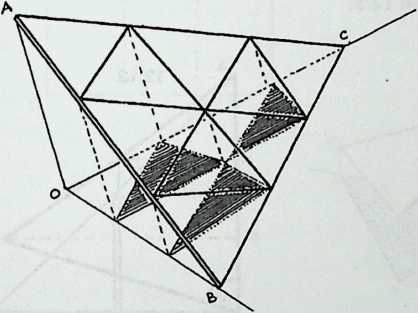
If we now look at the projection plane by itself (Diagram 12.7) we see that it is a right-angled triangle, and indistinguishable from the Cartesian and axes. Thus all points on the projected breakdown have simple integral coordinates, and so do the points on the octa face directly above them ( is at ).
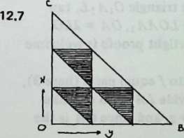
Diagram 12.8, a side view, shows how the slope of the octa face translates integral distances () from the origin into integral verticals (). Thus the coordinates of the breakdown vertices are also integral.
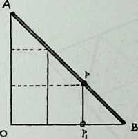
Turning now to Diagram 12.9, which is Diagram 12.6 redrawn with some details omitted, we see that the of point is simply . Its is . Thus is . Pythagoras tells us that hence .
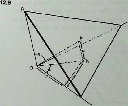
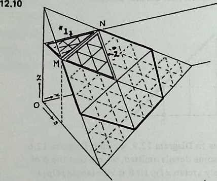
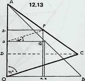
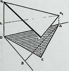
Before leaving the octahedron, we may recall A. J. Pugh’s observation that its truncated form, being a space-filling polyhedron, makes a sensible configuration to start from if we envisage clustered domes ((Polyhedra, University of California Press, 1976). The coordinates of truncated octahedral breakdowns are equally easy to write. Diagram 12.10shows why, to get a frequency (here ) we start from an octahedral subdivision of 3/ (here 9p). We divide the octa face edges into thirds and fold the top corner back until it is parallel with the projection plane; it will become a quarter of the square face, our triangle 1. Its and values remain as they were, but its parallelism with the projection plane makes its z retain everywhere the value of z along line , that is, (here = 6). Triangle 2 is a portion of the octa face, unchanged from its former orientation, so we can evaluate its points as if they were details in a 3/octa subdivision. Using our rule for writing the of single points, the reader can see that point 1 in Diagram 12.11 is at ; point 2 at ; point 4 at ; and so forth. And remembering to keep , he can identify point .4 as 0,1,6; point as ; and so on. Putting these values into the octahedron equations (Equation 12.1 and Equation 12.2) we can quickly derive the coordinates of all the points we need; thus is at .
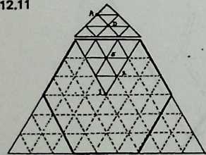
Diagram 12.12 shows what happens when we project an icosa face onto the plane where the Cartesian axes are located. The angle at the icosa apex makes the projection lie skew. In Diagram 12.13 we see the projection nestled between equal axes . The point is midway along ; we choose this special case to keep the diagram simple, but any point on the icosa face would do. is similarly located at the midpoint of . Its coordinates are , and we want to find the coordinates of . If , it is easy to see that ; ; and , as in Equation 12.4. Similarly, . But , so Thus , as in Equation 12.5.
For we turn to Diagram 12.14, which is the rear wall of Diagram 12.12, with the same lettering. is the icosa edge, is the axis with at the center of the polyhedron. We shall take for granted two facts inherent in the icosa’s governing ratios: that in the triangle , and that in the rectangle . (The reader with an appetite for airtight proofs is welcome to construct them.)
We now divide the icosa edge into equal parts (here 3), and by dropping perpendiculars divide and likewise. We remember that , and since is the -axis, and (again we are using a special case for simplicity). The into which we propose to convert this consists of two parts, the part in the triangle , the part in the rectangle . The former is , that is, . The latter is equivalent to , which is half ; but . Hence , as in Equation 12.6.
The tetrahedron is analyzed in the same manner, and the reader who wants proofs of Equation 12.10, Equation 12.11, and Equation 12.12 should have no difficulty working them out.
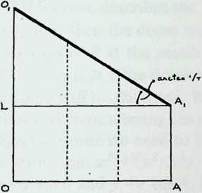
¶ Ellipses and Superellipses
So far we have acquired nothing, except some understanding, that couldn’t be contained in a comprehensive table of chord factors. The real interest of the spherical coordinates, making them worth the labor of computing them, is the way they facilitate geodesicizing nonspherical envelopes. The obvious profile to start with is the ellipse, and the most compact way of tackling the ellipse is to think of it as a member of a large family of shapes with a common mathematical description. We may look at the general equation first, and then move to simple cases by taking things out of it:
Here , and are ordinary Cartesian coordinates, at angles to one another; are any positive quantities you like. By varying them we can describe a surprising array of symmetrical shapes: a brick, a modified egg, a sphere, an octahedron (stretched or regular), a pair of crossed lines, a circle, any ellipse at all, not to mention various cigar shapes and squares with rounded corners. We may start in two dimensions by letting , which suppresses the third fraction entirely. Then if and are both 1, and and both 2, we get
which describes a circle centered at .
The radius of the circle, of course, doesn’t change. To get a changing radius we insert the terms and b. It is easiest to let a = 1 and take up all the variation in b. This gives us
which describes an ellipse. We see at once that if = 1 this equation is no different from that of the circle. Obviously determines how the radius varies as we travel round the curve. It is, in fact, the ratio (see Diagram 13.1) of the long and short axes, and to help ourselves remember this we may give it a name, , for expansion.
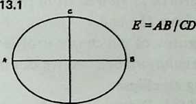
So the radius of the ellipse will vary between and 1, and an ellipse with an expansion of, say, 1.5 will be 1.5 times as long as it is broad. If this curve describes the profile of a dome with equatorial truncation, then the dome will have a radius of 1 at ground level and a radius of at the zenith. It is handy to let the floor radius ; then if the dome will be tall for its girth, and if the dome will be flattened. We can thus increase or diminish the headroom without altering the area of the circular floor.
To design the dome we need to know exactly how the radius varies. We know that , and from Diagram 13.2 we see that and . Inserting these values for and and rearranging, we obtain our first useful expression:
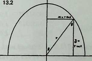
In Chapter 9 we calculated a very simple ( octa) dome using Equation 9.1, which gives us chord factors between two points of different radius. was 1.5, and we made a table in which one value had to be taken on trust. (It is now evident how it was arrived at.) For more ambitious cases we proceed in exactly the same way:
-
from the coordinate table, list the values of 0 that occur between the zenith and the truncation plane;
-
using Equation 13.1, obtain a value of for each 0; and
-
use Equation 9.1 to calculate the chord factors, being careful to use the proper pair of for each pair of s.
¶ Octahedral Ellipsoids
As usual, the octahedron is the easiest to handle. Its natural equatorial truncation keeps us out of trouble. Sliced at the equator, it yields a beehive shape with a circular floor. By slicing it down the long axis we obtain an elliptical floor, with a semi-elliptical profile as viewed from the side and a semicircular profile as viewed from the end.
Such figures, of which one profile is circular, are called ellipsoids of revolution, because we can imagine their being generated by twirling an ellipse.
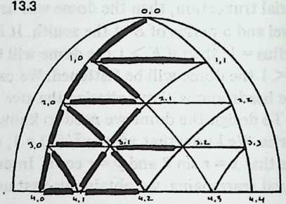
Example 7.1. Diagram 13.3 shows the coordinate diagram for a octa. For , the 6 values and radii are:
e |
r |
|---|---|
| 0 | 1.5 |
| 18.4349488 | 1.4142136 |
| 35.2643897 | 1.2602521 |
| 45.0 | 1.1766968 |
| 65.0051575 | 1.0497813 |
| 71.5650512 | 1.0289915 |
| 90.0 | 1.0 |
Chord factor 0,0/1,0 is obtained with Equation 9.1, using theradii
of 0,0 and 1,0 (1.5 and 1.4142136, respectively). It is 0.474423.
Fifteen more chord factors are calculated in this way, accounting
for every length in the left half of the diagram. Mirror symmetry
takes care of the rest.
Chord Factors
| 0,0/1,0 | 0.474423 | 2,1/3,1 | 0.696631 |
| 1,0/1,1 | 0.632456 | 3,1/3,2 | 0.606092 |
| 1,0/2,0 | 0.638578 | 3,0/4,0 | 0.326266 |
| 1,0/2,1 | 0.605791 | 3,0/4,1 | 0.454575 |
| 2,0/2,1 | 0.635872 | 4,0/4,1 | 0.320364 |
| 2,0/3,0 | 0.526758 | 3,1/4,1 | 0.452409 |
| 2,0/3,1 | 0.589150 | 4,1/4,2 | 0.459506 |
| 3,0/3,1 | 0.456607 | 3,1/4,2 | 0.532697 |
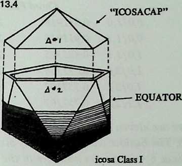 Icosahedral Ellipsoids
The five-way symmetries of the icosahedron make for especially
beautiful ellipsoidal patterns. This important advantage is its
principal one. As soon as we depart from spherical profiles, we
lose a virtue we have come to expect of the icosa, a relatively small
inventory of different strut lengths. Unless we are going to settle
for ridiculously shallow truncations, we must cope with two
different face triangles. This is clear from Diagram 13.4, where we
see the icosa dissected into (1) Fuller’s “icosacap,” the set of five
triangles surrounding the zenith, and (2) the set of ten triangles
around the waist. It is clear that we must enter this second set to
find the equator, and that the two sets will be stretched or
squashed in different proportions as the radius swings down. So
the icosa Class I tables provide coordinates for a second triangle.
In the same way, the icosa Class II tables cover five Class II tri-
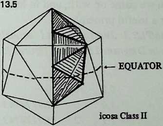 angles: Diagram 13.5 shows how they are located on the icosa.
We shall work an example from each class, and to keep the work brief we shall stick to 2v.
Example 7.2. 2v icosa Class II. Diagram 13.6 shows the vertex diagram for the five Class II triangles. The coordinates are quickly listed from the table, and the radii calculated:
e |
r |
||
|---|---|---|---|
| 0,1 | 0 | 0 | |
| 1,0 | 0 | 37.3773681 | 1.2411302 |
| 1,1 | 72 | 37.3773681 | 1.2411302 |
| 2,0 | 0 | 79.1876830 | 1.0099209 |
| 2,1 | 36 | 63.4349488 | 1.0606601 |
| 3,0 | 0 | 116.5650512 | 1.0606601 |
| 3,1 | 36 | 100.8123170 | 1.0099209 |
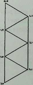 The symmetries above and below the line are evident from the
13.6
table of radii above: 2,0 corresponds with 3,1 and 2,1 with 3,0. To
see how this works out in distances, we shall this time list all the
chord factors:
Chord Factors
| 0,0/1,0 | 0.911918 | 2,0/2,1 | 0.665207 |
| 0,0/1,1 | 0.911918 | 2,1/3,1 | 0.665207 |
| 1,0/1,1 | 0.885725 | 2,0/3,1 | 0.720724 |
| 1.0/2,0 | 0.831758 | 2,0/3,0 | 0.665207 |
| 1,0/2,1 | 0.757107 | 3,0/3,1 | 0.665207 |
| 1,1/2,1 | 0.757107 |
There are eleven distances in the diagram, but only six different ones. The builder would need only six different members.
Since occurs nowhere in the coordinate table, no point on this structure lies on an equator. Indeed, we may wonder how we should go about truncating it. Chapter 14 will tell.
We move on to the second icosa example, a Class I ellipse. This time we shall use a fractional expansion, , to get a saucer rather than a beehive. We shall have fault to find with the first version we come up with, and in learning how to modify it will master a useful principle.
Example 7.3. 2v icosa Class I, squashed. The coordinate layout is shown in Diagram 13.7. The figures look like this:
0 |
r(E = 1/1.5) |
||
|---|---|---|---|
| 0,0 | 0 | 0 | 0.66666667 |
| 1,0 | 0 | 31.7174743 | 0.72461704 |
| 1,1 | 72 | 31.7174743 | 0.72461704 |
| 2,0 | 0 | 63.4349488 | 0.89442719 |
| 2,1 | 36 | 58.2825255 | 0.86210372 |
| 3,1 | 18 | 90.0 | 1.0 |
| 3/2 | 54 | 90.0 | 1.0 |
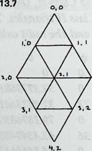
Though the coordinate table goes past and , we don’t need any values beyond (the equator). We now compute chord factors and get the following:
0,0/1,0
1,0/1,1
1,0/2,0
1.0/2,1
0.384256
0.447838
0.471622
0.507459
2,0/2,1
2,0/3,1
2,1/3,1
3,1/3,2
0.481007
0.527551
0.590178
0.618034
¶ Modifying Coordinates
Study of the chord factors we have just calculated, or better still study of a simple model, will disclose an unwelcome asymmetry: the short members are bunched around the zenith, where they have little to contribute but weight, and the longest members, straddling the most widely separated vertices, are found around the sides where the load is being transmitted to earth. A glance at Diagram 13.8 shows what has happened. Our coordinate system was designed to give reasonably uniform member lengths on a sphere. When a shallow curve intercepts the bundle of sight lines, different struts are differently affected. This is true of course with any non-circular contour, but it is more likely to be troublesome with a shallow ellipse. A beehive may often concentrate its elongations near the zenith with neither aesthetic nor structural harm, since the zenith members have little load to bear.
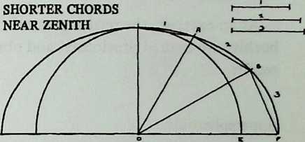
Our recourse is to modify the coordinates before doing anything else. Instead of projecting the array against an expanded envelope, we might in effect allow the expansion of the envelope to pull the zenith coordinates apart. This is like reflecting the array off a slanted mirror whose slope is governed by the expansion (Diagram 13.9). Each is replaced by , obtained from
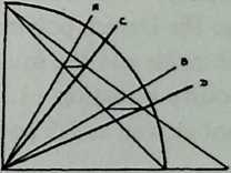

Diagram 13.10 shows a typical result. The stretching of chords now tends to parallel the long axis of the ellipsethe reverse of the situation in Diagram 13.8— and the zenith of a shallow structure is no longer congested with short members. Calculation would also show that the overall variation in strut length is reduced. This procedure gives chord factors identical with those of the elliptical structures in Domebook 2. We may nickname it the E Correction.
But there is a simple way to do still better. Replace each by , obtained from
We may call this the Root E Correction. It distributes the strut lengths very much as the parent sphere did, the longest members part-way down, shorter ones toward zenith and base. And the overall variation of strut lengths is held within close boundsprobably the closest we can easily obtain. In fact the Root E Correction may be recommended as a routine procedure for all elliptical geodesics. For the case we have been discussing it gives these chord factors:
| ,0/1,0 | ,0/2,1 | ||
| ,0/1,1 | ,0/3,1 | ||
| lj0/2,0 | ,113,1 | ||
| ,0/2,1 | ,1/3,2 |
As an exercise, the reader may refigure the Class II icosa beehive we figured previously, and observe the improvement that results.
¶ Superspheroids
At the beginning of this chapter we displayed a general equation from which we obtained the equation of the circle by assigning appropriate values. To the two exponents and we assigned the value 2, and we kept 2 for an exponent when we went on to the ellipse. But there is no reason any exponent needs to be 2. It can be anything from zero to infinity. If it is zero, the ellipse or circle equation yields not a curve but a pair of crossed lines. If it is infinity, we obtain a rectangle (or, if , a square). Some years ago the Danish polymath Piet Hein proposed mediating between the circle and the square by making the exponent 2.5. If we modify Equation 13.1 in this way, remembering to insert a 2.5 root as well as 2.5 powers
we have once again a formula for a varying radius, that of a
supercircle if , and of a superellipse if has some other value, for instance 1.5.[9] The supercircle radius formula by itself looks like this:
A supercircle (Diagram 13.11) is beginning to develop shoulders. A superellipse (Diagram 13.12) has less taper than a normal ellipse of the same expansion. A dome with either profile retains more of its headroom further from the center than does the non-super version. The versatile Peter Calthorpe designed a superspherical icosa some years ago. The one effort I know of to build one encountered legal and financial troubles unrelated to the design.
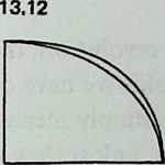
The simplest way to use these shapes is to combine them with a circular floor plan as we did the ellipse. We thus obtain the shape generated by twirling a supercircle or a superellipse on its axis: a superspheroid or a superellipsoid of revolution.
The (or y*) function on the calculator makes 2.5 almost as easy an exponent to use as 2. (We get the 2.5th root by raising to the power ). Radius tables and then chord factors are obtained exactly as they were earlier in this chapter. The reader should have no difficulty obtaining the following chord factors for a octa supersphere:
| ,0/1,0 | ,0/3,1 | ||
| ,0/1,1 | ,0/4,0 | ||
| ,0/2,0 | ,014,1 | ||
| ,0/2,1 | ,1 /4.1 | ||
| ,0/2,1 | ,014,1 | ||
| ,0/3,0 | ,114,2 | ||
| ,0/3,1 | ,114,2 | ||
| ,1/3,1 | ,1 /3,2 |
Two of these are duplicated, so the octa supersphere requires 14 different components, as against 6 for a normal sphere. Careful study of a model is the only way to decide if it is worth the complication.
Just as 2 is an optional exponent, so is 2.5. The latter has no special magic except that Piet Hein likes the curves it generates. By raising the supersphere exponent to 3, we can retain headroom even further from the center, But another way of putting this is
that we are making a large area around the zenith nearly flat (see Diagram 13.13). The spherical excess of the structure is concentrated in a rather narrow zone where roof suddenly becomes wall. Nearly flat areas in geodesic structures are areas of potential trouble, requiring careful hub detailing to retain the integrity of the tension network. Stretching the supercircle into a superellipse expands the problem area, and exponents above 2.5 are not recommended for superellipses.
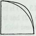
¶ Varying Two Radii
The sphere is a circle of revolution; the supersphere is a supercircle of revolution; the ellipsoids we have considered have been ellipsoids of revolution. This simply means that one cross-section is circular, and such domes, unless they are truncated obliquely, will have either a circular floor plan and a special profile, or a special floor plan and one semicircular profile. The structure’s native sphericity is expanded (or contracted) in only one direction.
But there is no reason why we cannot vary two radii. This means specifying two separate expansions, and , one for the floor and the other for the profile. (Separate need not mean different both expansions may have the same value, but they will both make their presences felt.) So we could have a supercircular profile, to get headroom, and a superelliptical floor plan, to get walking space. The respective expansions would be 1 and something else, say 1.25. The exponents could be the same, or different. The structure would have no circular cross-section at all.
Since the radius of each vertex is now responding to two expansions, and perhaps to two exponents, the arithmetic becomes more labyrinthine. Still, all we need to calculate chord factors is a table of radii as measured from a central point, and we can make one if we keep our heads.
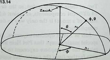
Diagram 13.14 shows the situation. We want the radius from the center of the system to vertex . We first assume a floor plane passing through the center (though when we are finished nothing will prevent us putting the floor somewhere else). We next want which is the radius of the floor at the point where the meridian through the vertex in question crosses its edge. This radius is a function of , the expansion of the floor ellipse, and of the of the vertex in question. Its equation is:
We might tabulate for every pertinent value of 0, which means for one-quarter of the dome’s perimeter, and use it to obtain r2, the radius we want for chord factors, as follows:
But we should go to all this trouble only in the unlikely case when we might want to use different values of the exponent for the two radii. The exponent is, of course, 2 for ellipses and normally 2.5 for super circles and superellipses, and it seems ill-advised to mix the two in one structure. So we take advantage of the fact that when the two exponents are identical the two equations collapse into one:
(The exponent , if you’ve forgotten, means the th root.)
For high jinks of this kind the octahedron has obvious advantages, since one face triangle takes care of the whole quadrant and brings us clear down to the equatorial truncation line. In Chapter 15 we shall look at its disadvantages, which stem from the way its tendency toward flatness at the square vertices is accentuated by the flat areas peculiar to the superellipse.
The icosa remains elegant and far from impossible. In Chapter 15 we shall develop a fancy application in detail, and a worked example is deferred until then.
A few pages back we found that it was sometimes desirable to improve the symmetry of a non-spherical form by modifying one coordinate; Equation 13.2 gave a convenient method. Now that we are dealing with two expansions the symmetry has more ways of becoming displeasing, and improving it will mean modifying both coordinates. An elegant result is obtained by changing 0 to 0p:
and to .
These expressions reproduce the effect of projecting points onto a sphere and then expanding it, rather than projecting spherical coordinates onto an already expanded envelope. The designer will have to judge whether they are worth the bother.
They assume, too, that the floor is being expanded along the axis, an innocuous assumption if we are using the octahedron, whose and axes are indistinguishable. Chapter 15 shows that with the icosahedron there is reason to make a decision, and should we decide to expand its floor along the axis, we need to alter both equations slightly. In Equation 13.8 the division becomes a multiplication, and in Equation 13.9 “” and “” must be interchanged.
¶ Free Forms
It is possible to apply the geodesic three-way grid to any surface that can be mathematically described. The description is not always easy, and one can conceive of convex curves that would give a skilled mathematician trouble. One thing that is simple in spherical coordinates, though, is the notation for any surface of revolution whose profile is a convex curve drawn freehand. Should you want a shape like the one in Diagram 13.15, you have only to draw it on graph paper, designate an origin point, and from that point run radii out to the curve, the angle of each radius with the vertical axis being one of the values for the breakdown you have chosen. Call the length of the vertical axis , and measure the other radii. Then use those radii, and the values from the table for your breakdown, in Equation 9.1 to get chord factors. The octahedron’s seams make it possible to combine two such profiles, left and right. Keep the roofline convex and avoid extended arcs of very low curvature, unless you are prepared to take the structural measures described in Chapter 16.
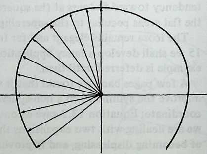
¶ Truncations
So far we have been accepting symmetry systems just as they come from the mathematician’s repertory. We made certain choices: the rest was law. We chose a polyhedron, we chose a frequency and a breakdown, we chose floor and roofline cross-sections with an expansion and an exponent for each; having chosen, we accepted what came out of the calculator. It is now time to contemplate a few interventions, which modify the crystalline symmetry of the result to make it more useful. In particular, we want to be able to slice our complex polyhedron at will and make it sit flat; we need to design truncation planes into it.
A few of these are inherent, and always equatorial. The octahedron has natural equators, the inherent great circles, and any breakdown preserves some of them. Complete icosahedral great circles are preserved by any even-frequency Class I breakdown. Class II icosa great circles are tantalizing: they are twice interrupted in their circuit around the sphere, and they lie flat only when the sphere is tipped so that an edge, not a vertex, is at the zenith. To get at them will take special handling: we’ll come to that.
If we want something other than a hemispherein short, a lesser-circle truncationvie find that no combination of breakdown and frequency will give it to us. We shall have to tamper.
There are two main ways of tampering. One is to devise a truncatable breakdown, which supplies crisscrossing lesser circles throughout the system. Any of these will then serve as a truncation plane. Diagram 14.1 gives a rough idea. In its raw state the icosa is girdled by twelve approximate lesser circles, running in pairs like the Tropic of Cancer and the Tropic of Capricorn, parallel to six imaginary equators (the six great circles, which the breakdown does not incorporate). They are so nearly level that many builders have simply chosen to pretend they were truncation planes, and have shored up the wobble with blocks (see Lloyd Kahn’s Domebook 2 [Bolinas, Ca., Pacific Domes: 1971] p. 24). Truncatable breakdowns level all twelve of these circles off, giving the builder a choice of two genuine truncation planes, at approximately and of the sphere’s volume.
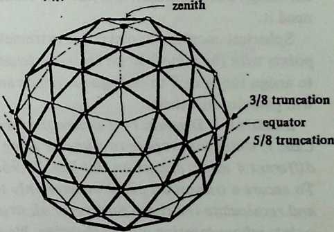
This attractive method leads to a couple of interrelated difficulties. Tampering with the overall geometry can lead to poor distribution of spherical excess; avoiding that can lead to surprisingly wide variations in strut length. Some of the earliest truncatable designs incurred the first of these difficulties: the pentagon vertices were excessively peaked, leaving the rest excessively flat. Other solutions trade asymmetry of spherical excess for asymmetry of member length, chord factors varying as much as 45 percent (vs. about 17 percent for the normal 3p). Truncatables do not need to be unhandsome: an especially fine roofs the religious center at the Edwardsville campus of Southern Illinois University, strut lengths varying in a sequence so elegant it looks more like an aesthetic modulation than an engineer’s contrivance {Architectural Forum, January-February, 1972:86, fig. 5).
Still, for many purposes the second main solution to the truncation problem is preferable. It amounts to leaving most of the design alone and inserting just one truncation plane where we need it.
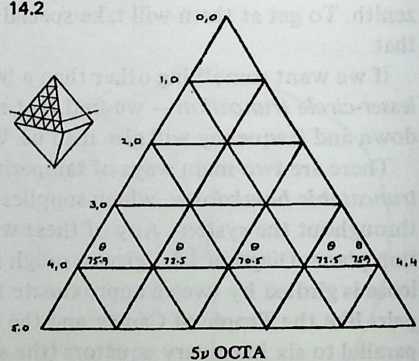
Spherical coordinates make this extremely simple. Since all points with the same 6 lie on the same lesser circle, we have only to assign the same to contiguous points and a truncation plane will pass through them.
Example 8.1. Diagram 14.2 shows one face triangle of a 5v octa, Class I, which we propose to truncate along the line 4,0-4,4. Three different values appear on this line, 75.9638, 72.4516, 70.5288. To secure a truncation plane we have only to make them all equal and recalculate the chord factors for all struts connected to the points whose location we are changing. We can select one of these values say, the edge oneand make the others like it, or we can arbitrarily bring everything to some convenient normsay, 72. In any case, since the bottom row (5,0-5,5) will be discarded in the truncation process, and mirror symmetry takes care of the right half of the system once we have determined the left, this means, at most, recalculating just 6 values: 3,0/4,0; 4,0/4,1; 3,0/4,1;/4,2; 3,1/4,1; 3,1/4,2. Everything else is left as it was.
The icosa as usual requires a little more care. What Fuller calls the icosacap (the five triangles around the zenith) makes so shallow a saucer we are unlikely to want to use it by itself, let alone truncate it. Icosa truncations will cut through the 10 triangles that girdle the sphere’s waist, the #2 triangles in the diagram we took into account with ellipsoids in Chapter 13.
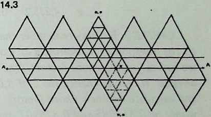
Diagram 14.3 shows a Class I icosa opened out to display all twenty face triangles. A likely plane of truncation would follow line , passing below the equator to give the so-called truncation. Inspecting the Class I icosa tables, we see at once why amateur builders have gotten by with this truncation as it stands, using blocks to shore up the discrepant places: along the line 4,1-4,3, which is where we are cutting, the 0 values luckily differ by only 2/3°. To achieve a perfect truncation, we have only to raise the 9 of point 4,2 from 79.1877 to 80.1169 and refigure the associated chord factors. (We might elect instead to leave 4,2 alone and bring 4,1 and 4,3 into agreement with it, but then we should also have to alter 5,2 and 5,3 on the down-pointing adjacent triangles to make them match. It saves work to leave edge points alone when we can.)
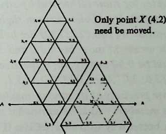
So many icosa domes with uneven -sphere truncations have been built from Domebook data that full data for a smooth cutoff may be interesting. The basic chord factors are:
| a | 0,0/1,0 | 0.348615 |
| b | 1,0/1,1 | 0.403548 |
| c | 1,0/2,1 | 0.412411 |
| d | 1,0/2,0 | 0.403548 |
These are used for the five top (icosacap) triangles. They are also used for the #2 triangles that point downward below them; for a truncation the down-pointing triangles are completed as far as . It is on the up-pointing #2 triangles flanking them that we move to its new position , making its equal to that of and (that is, ). With this we obtain new chord factors for and :
| e | 4,2/4,1 | 0.412703 |
| f | 4,215,2 | 0.398734 |
These are used only for the members around the truncation perimeter; for the rest of the dome we use regular chord factors.
If we wanted a 3/8 truncation instead of a truncation, study of the diagram shows that we should use a revised chord factor for instead of . It is
| g | 4,2/5,2 | 0.426214 |
Example 8.2. We may remember that we left dangling in Chapter 13 the question of truncating a 2v icosa Class II ellipse for which we had calculated chord factors. One way of doing this is now obvious. We could change the 0 of 3,0 to agree with that of 3,1 and calculate two new chord factors, 3,0/3,1 and 2,0/3,0. These would be 0.613085 and 0.378907, respectively. The latter figure provides for some rather stubby structural members, but the dome will sit flat. It will also curve in slightly near the bottom, since the truncation 6 (100.8123170) lies below the 90° line.
Or we might move both 3,0 and 3,1 up to 90° (their coordinates would be 0,90 and 36,90, respectively) and refigure four distances: 2,0/3,0; 2,0/3,1; 3,0/3,1; 2,1/3,1. This would truncate the ellipse precisely at its zone of maximum radius, though all the base members would be somewhat short.
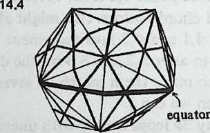
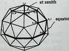
A better way to truncate Class II spheres introduces us to a new principle:
¶ Truncation by Rotation
While we were struggling with the last example, the reader may have been wondering what happened to the great circles to which Class II breakdowns give access. The answer is that they are ready and waiting, but not while a vertex is at the zenith. Diagram 14.4 shows this; if we rotate the structure till an edge is on top we obtain equatorial great circles, twice interrupted in their circuit of the sphere.
Since the whole coordinate system hangs together, what we need is a way of rotating it as a whole until the midpoint of an icosa edge moves to the zenith.
The midpoint of a Class II icosa edge is . This is listed in the Chapter 21 tables as Point 2,1 of a Class II breakdown. If this isn’t clear, consult Diagram 10.6, which shows the icosa edge passing down the middle of a Class II triangle. We need a way of telling what the other points become when this point becomes 0,0. We use the rotation formulae[10], which tell us that when 0,0 moves to 0,0, then will move to:
and will move to:
Let us try this out with a Class II sphere. The Class II Method 1 tables give us the following coordinates for an icosa:
| ,0 | ||
| ,0 | ||
| ,1 | ||
| ,0 | ||
| ,1 | ||
| ,0 | ||
| ,1 |
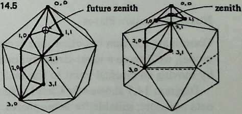
We can see from Diagram 14.5 that when a structure is rotated in the manner we contemplate, 3,0 will lie on the equator and 3,1 somewhere above it. Clearly these are the only points that will have anything to do with a truncation, so we ignore all the others and feed these two into the rotation formulae. We obtain, if we use 36 for and for , the following new coordinates:
3,0 -31.717474 90
. 3,1 0 69.0948426
We will have a truncation if we create a new vertex, 0,90, for the center of the diamond we are slicing and join both these points to it. The point can be called , and the chord factors will be:
3,0/x 0.546533
3,1/x 0.362843
This will give us an edge-zenith sphere with a truncation utilizing one of its inherent great circles. The regular chord factors will take care of all the other structural members.
This particular problem could be solved in perhaps less time geometrically. But at higher frequencies than , coordinate rotation is the way to solve Class II truncation problems. The diamond being sliced by the truncation plane has always the same boundaries; at higher frequencies we are simply inserting more new members (Diagram 14.6).
It would be quite possible to handle the Class II ellipse in the same way. We should first rotate all the coordinates, then obtain radii, chord factors, and truncation members. The method is not recommended for three reasons:
-
It is a great deal of work.
-
An ellipsoid with an edge zenith is an awkward looking structure.
-
By the time we have finished the coordinates have undergone so much manipulation that rounding-off errors make the fifth place of the chord factors wobbly.
¶ Novel Truncation Planes
Coordinate rotation has other uses. Occasionally, examining a model, we discern a lesser-circle truncation plane made available by moving an unusual point to the zenith.
Diagram 14.7 shows a Class I octa sphere. It has the usual octa equators, suitable for hemispheres. Rotating a model, however, till the central vertex of an octa face (2,1) is at the zenith, we notice two irregular lesser circles, resembling those of the icosa.
Truncation along the lower one of these is ah interesting possibility. The resulting structure is somewhat taller than a hemisphere and has three quadrangular skylights symmetrically disposed around the zenith.
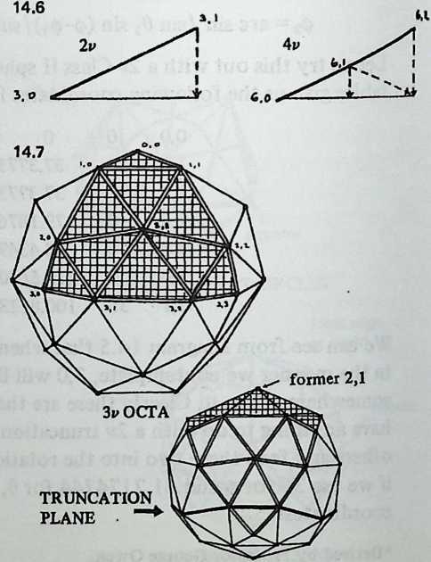
Our first step, clearly, is to make the coordinate system correspond with the way we are viewing the model, by moving 2,1 to the zenith. We won’t, of course, be calculating the result of moving every pointjust the ones that will be affected when we straighten out that lesser circle. Diagram 14.8 shows the situation. Rotating the sphere toward the eye until the 2,1 point on the far side arrives at the zenith, we discover that the array on the face nearest us has moved down to the desired truncation plane, which is irregular because 2,1 is misaligned with its neighbors. To straighten out the truncation plane we have only to equalize the values these three points assume in their rotated position. We shall be altering the occupied by a shifted 2,1, and shall need its revised distances from a shifted 2,0 and a shifted 1,0. So we need rotate only these three points.
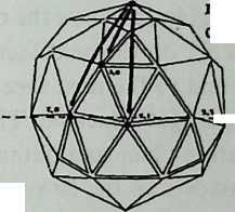
The coordinates of the point on the far side of the sphere, which we propose to move to the zenith, are 225, . (Its is the same as that of 2,1, and its 0 is 180° greater.) Inserting these figures into Equation 14.1 and Equation 14.2 along with the coordinates of the three points to be recalculated, we obtain their new coordinates:
| 1,0 | ||
| 2,0 | ||
| 2,1 |
As we might have expected, the new of 2,1 is relatively close to that of 2,0 (and by symmetry, of 2,2). To effect the truncation, we equate them, taking the edge-point value (104.9632174) as the norm. Using this new value for 2,1 we obtain the following revised chord factors:
2,0/2,I 0.674981
1,0/2,1 0.607864
Being very careful to notice what goes where (Diagram 14.9), the builder how employs these values in zones adjacent to the truncation plane and constructions a rotated/truncated octahedron with 2,1 at the zenith. The disposition of the square skylights is pretty.
For a more tightly woven mesh, we might double the frequency of this. For a we would straighten out the row 4,0-4,1-4,2-4,3- 4,4. Mirror symmetry permits us to do this by attending only to and 4,2 plus the points connected with them, 3,0 and 3,1. But (see Diagram 14.10) the 2,1 point on the adjacent, down-pointing octa face is now located on the truncation plane and must be aligned with its neighbors. When the octa was in its unrotated position, this was 5,1 on the next face clockwise; take the 0 of 5,1, add 90° to get round to the next face, and relocate the result like the other points that get relocated. Then give it the same 0 as the rest of the truncation plane and obtain new chord factors.
The square windows on the version will be smaller than on the . Should we prefer the larger size, we could omit 1,0 /1,1, 1,0/2,1 and 1,1 /2,1, then figure 0,0/2,0 and 2,0/2,2 as a single long chord.
Should we like this well enough to attempt an elliptical version, we should need to move more points: Diagram 14.11 shows where they are located.
¶ Zenith Altitude and Floor Radius
Having truncated a dome we shall want to know how high its zenith point will be and how large its floor. Diagram 14.12 shows the derivation of two very simple formulas. The zenith altitude is simply:
altitude = - cos 0, [Eq. 14.3]
and the floor radius is given by:
floor radius = sin 0. [Eq. 14.4]
In these expressions is of course the 6 of the truncation plane, and for spheres = 1. So for the rotated octa discussed previously, the zenith altitude is 1 - cos 104.9632174, or 1.258199, which means we have gained 25 percent more zenith headroom than a hemispherical truncation would have permitted, and the floor radius is sin 104.9632174, or 0.966092. The floor area is approximately , or 2.932153 (“approximately” because we are pretending a polygon is a circle); since the floor of a hemisphere (radius = 1) would be 3.141593, we have gained our extra headroom at a cost of 6.66 percent in floor area.
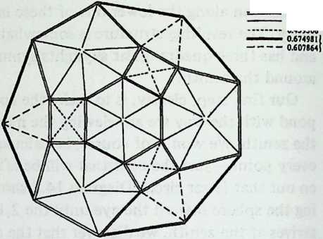
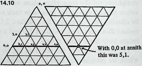
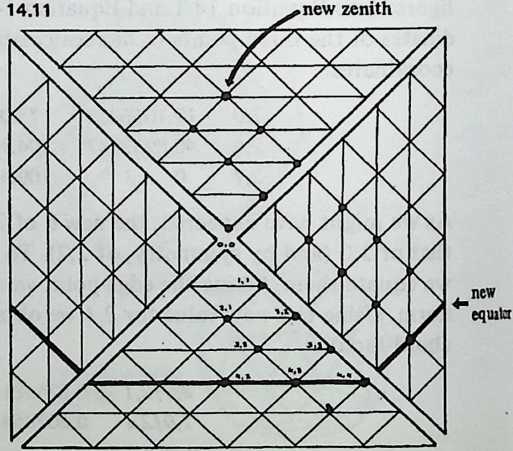
Should we be analyzing elliptical contours, we should need slightly more complicated expressions: if is the radius of the zenith point, and is the radius at the truncation plane, then
altitude = rz - rt cos 6. [Eq. 14.5]
floor radius = rt sin 6. [Eq. 14.6]
If the floor is itself elliptical, there will be numerous values of ; we should probably be interested in the largest and the smallest, which would give us the length and width of the floor.
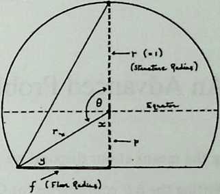
¶ An Advanced Problem
Among the means at our disposal we may now list the following:
-
Writing the 0,6 coordinates for Class I or Class II breakdowns of icosa, octa, or tetra polyhedra (Chapter 12, data in Part 3).
-
Obtaining the distance (chord factor) between any two points on a spherical contour (Equation 9.2).
-
Writing the third coordinate, r, for any 0 when the floor plan is circular and the silhouette is elliptical or superelliptical (Equations 13.1, 13.3, 13.4).
-
Writing the third coordinate, r, for any 0,0 when both floor plan and silhouette are elliptical or superelliptical (Equation 13.7).
-
Correcting for uneven expansion (Equations 13.2, 13.8, 13.9).
-
Obtaining the distance (chord factor) between any two points on a nonspherical contour, once we have their three coordinates 0, 0, and (Equation 9.1).
-
Inserting truncation planes at will (Chapter 14).
-
Rotating the coordinate system to bring any point to the zenith (Equations 14.1,14.2).
We may now want to tackle a sophisticated problem that tests our resources. The harvest of insights seems to be worth the few pages we shall need to work it out in full. The reader who wants to test his command of the equations can spot-check any result at any point.
Near the end of Chapter 13 we were considering a superelliptical floor plan and contour, with a supercircular cross section. This offers the advantage of considerable floor space, with headroom maintained well out from the center. Because it is symmetrical by quadrants, it invites the use of the octahedron, one face triangle of which yields one quadrant exactly.
Unfortunately, it compounds a defect of the octahedron, deficient spherical excess at the principal vertices. If we are standing inside an octahedral geodesic hemisphere, a four-way vertex is directly overhead. If the breakdown is 4-frequency, the radials of this vertex will have chord factors of 0.141778, bounded by a square whose sides are 0.200000. These are almost right-angled triangles; the four angles meeting at the vertex are each 89.7121°, alarmingly close to the 90° which would make this vertex perfectly flat. Octahedral spheres are feasible because the small flat area is fully surrounded by vertices whose departure from flatness is correspondingly more emphatic. There is nothing wrong with flat vertices properly distributed. Fuller himself pioneered the hexpent configuration, which replaces pentagonal and hexagonal arrays with flat plates, in effect flattening numerous vertices throughout the system and relying on surrounding tensional grids to hold things together, and numerous hex-pent radomes have been withstanding Arctic winds on the DEW line for many years.
But once we introduce the superspherical or superelliptical contour, we find that quasiflatness is creeping a considerable distance out from the zenith. Not only is the zenith of the octa nearly flat, but so are the four vertices around it. Try the icosa- hedron. The angles around the pent vertex of a sphere are each 71.3316°, so five total 356.658°. The four octa angles totaled 358.848°, so the icosa is helpfully less flat.
Now try it with the superellipse. We shall be using the same parameters throughout this chapter: floor expansion, 1.5; roofline expansion, 1,0; both exponents, 2.5. Above the superelliptical floor, we have a supercircle profile in one cross section, a super-ellipse profile in the other. So if the pent vertex overhead has a radius of 1, the 5 vertices surrounding it have radii greater than 1, pushing the ends of the radials out toward flatness. Calculating radii and chord factors, we find that the. 5 pent angles are each 71.985°, or 359.925° for the setvirtually flat.
Moreover, we have quadrant symmetry, and the icosa with its 72° radials will be awkward to quarter.
The solution, discovered by Bill Wild of Vail, Colorado, whose results appear without commentary in Shelter (Bolinas, Ca.: Shelter Publications, 1973) p. 126, is to move the icosa vertices away from the zenith. Move an edge to the zenith, and let it follow the super circular profile, so that the pent vertices at its ends will be carried down to where curvature is accentuated. Then instead of having less spherical excess than when the envelope is a sphere, they will have more. And overhead there will be no vertex at all to suffer that undue flatness (Diagram 15.1).
There is a bonus. With an edge up, the icosa will quarter neatly, the cuts running along that edge and straight down the centers of face triangles.
To achieve this we do the following:
-
Discover how much of the icosahedron we shall need to account for, to include all points in a quadrant of a hemisphere.
-
Write the coordinates of these points.
-
Rotate the system of coordinates till the center of an icosa edge is at 0,0.
-
Obtain the radii of all points in this new position.
-
Obtain the chord factors.
-
Attend to any truncation problems.
¶ Quartering the Icosa
Diagram 15.2 shows the situation. The icosahedron is edge-upward, and the fifteen great circles are marked on it. Their 90° intersections at face-triangle edges give us just the demarcations we want; as the diagram shows, a full icosa triangle plus halves of three others will exactly cover one quadrant of a hemisphere. (This makes 2 1/2 triangles, and since 4X21/2=10, our result agrees with the fact that 20/2 =10 icosa triangles would constitute a hemisphere.)
¶ Writing the Coordinates
Look at Diagram 15.3. The line 0,0-4,0 is the edge that will move to zenith. The full triangle we want is the second icosa triangle in the tables, 4,0-4,4-8,4. Of the upper icosa triangle (0,0-4,0-4,4) we need only half, as shown. Since two struts pass across its upper boundary, we also need points 2,1 and 3,3. All these points are obtained directly from the tables. 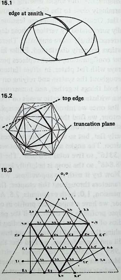
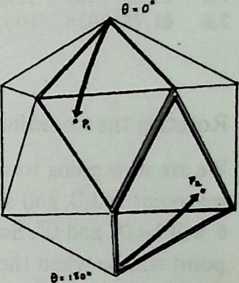
To obtain coordinates for the part-triangles 4,0-8,2-8,4 and 4,4-8,4-6,6 we remember how the icosa is put together (see Diagram 15.4). These are also second triangles, but up-pointing. Any point in them will be the same distance from the bottom icosa vertex (0 = 180°) as the corresponding point in the usual second triangle is from the top vertex (6 = 0°). So we identify corresponding points and subtract from 180°. Thus 7,2 corresponds to 5,2; subtracting the 0 of 5,2 from 180°, we obtain a 0 for 7,2: 106.0450570°.
To obtain the 0 values of these points, we note that symmetry places them left and right of icosa-triangle centerlines exactly as the corresponding points in the second triangle are placed left and right of its centerline. Its centerline is at 0 = 36°. The up-pointing triangle centerlines are at 0 = 0° and 0 = 72°. Since 5,2 is 36° - 26.2676986° = 9.7323014° from the 36° centerline, the 0 of 7,2 is 0 + 9.732014 = 9.7323014°, and the 0 of 7,5 is 72 - 9.7323014 = 62.2676986°.
Again notice that edge-crossing struts will require us to write some coordinates outside these boundaries. Since 5,0 and 7,1 are to the left of the 0 = 0 line, their 0 values are negative. Table 15.1 lists all of the coordinates we require.
TABLE 15.1 Coordinates from Table
| 0 | fl | ||||
| ,0 | ,1 | ||||
| ,1 | ,2 | ||||
| ,0 | ,3 | ||||
| ,1 | ,4 | ||||
| ,2 | ,5 | ||||
| ,3 | ,1 | ||||
| ,0 | ,2 | ||||
| ,1 | ,3 | ||||
| ,2 | ,4 | ||||
| ,3 | ,5 | ||||
| ,4 | ,6 | ||||
| ,0 | ,1 |
| 0 | |||||
| ,2 | ,2 | ||||
| ,3 | ,3 | ||||
| ,4 | ,4 | ||||
| ,5 | ,5 | ||||
| ,6 |
¶ Rotating the Coordinate System
We are now going to move the midpoint of the edge 0,0-4,0. This midpoint is 2,0, and since it will now occupy the zenith, its 0 and 0 will be 0° and 0°. So we want to know what the 0 and 9 of each point will be when the present 0, 31.71747438 has been moved to 0,0. Equation 18.1 and Equation 18.2 give us the answers, with tedium but not difficulty. One caution is needed: we must watch that we assign 0 to the right quadrant. Diagram 15.5 shows the new boundaries: normally all values will lie between 0 and 90. Thus 8,5 and 7,6 are the only points below the equator. Here Equation 14.1 will give us the proper 9 values. Point 2,1, however, lies beyond 0 = 90°, and here we confront the fact that Equation 14.2 yields its answer as an arcsine, in this case arcsine 0.8506508. The unthinking answer is 58.2825260. But we need something greater than 90°; the value we want must be in the second quadrant, 121.7174740. Similarly, the 0 values for 5,0 and 7,1 must be negative but not a great deal less than zero: they are in fact the negative values of their counterparts 5,1 and 7,2. An eye kept on the diagram’s physical realities will prevent mistakes.
Table 15.2 shows the rotated coordinates. To prevent confusion the points keep their old labels.
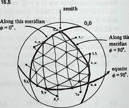
| TABLE 15.2 | |||
| 0 | r | ||
|
|||
|
|||
|
|||
|
| 0 | |||
| ,2 | |||
| ,3 | |||
| ,0 | |||
| ,1 | |||
| ,2 | |||
| ,3 | |||
| ,4 | |||
| ,0 | |||
| ,1 | |||
| ,2 | |||
| ,3 | |||
| ,4 | |||
| ,5 | |||
| ,1 | |||
| ,2 | |||
| ,3 | |||
| ,4 | |||
| ,5 | |||
| ,6 | |||
| ,1 | |||
| ,3 | |||
| ,4 | |||
| ,5 | |||
| ,6 | |||
| ,2 | |||
| ,3 | |||
| ,4 | |||
| ,5 |
If we intend to alter the coordinate symmetry with the help of Equations 13.8 and 13.9, now is the time to do it. To shorten the example we’ll skip this option, remarking only that since the floor is being expanded along the 0 = 90° axis, both equations would require the modification explained previously.
¶ Tabulating the Radii
Again the work is tedious but perfectly straightforward. There is only one thing to remember: the direction of the long axis of the floor. With a vertex at the zenith the usual situationthis is unimportant, but here we want to be sure that the vertexial edge runs along the supercircular rooftree, not the superelliptical one. This is chiefly to work the pent centers at the ends of this icosa edge as far down into the zone of curvature as we can. (It also happens to yield a tighter clustering of chord factors.) Now Equation 13.5 as it stands will expand the floor along the axis, which is 90° from where we want it. The easiest way to swing things 90° is to alter Equation 13.7 very slightly; we have only to interchange and , and Equation 13.7 will swing the floor plan as we want, and generate the radii as tabulated in the right-hand column of Table 15.2.
¶ Chord Factors
This is the ungrateful case where symmetry fails us on any scale smaller than 1 /8 sphere; hence, we need chord factors for all the struts in the dome quadrant. A good way not to miss any is to mark each strut red on a diagram as its value is computed.
Equation 9.1 will give the values in Table 15.3. They do not correspond to those shown by Mr. Wild in Shelter because his expansion was only 1.25, while ours is 1.5. A model will tell us whether we like the looks of it; if not, we can go back to Mr. Wild’s stubbier form. (Refigure radii, refigure chord factors.)
TABLE 15.3 Chord Factors
| ,0/3,0 | ,1 /5,1 | ,2/6,2 | |||
| ,0/3,1 | ,1/5,2 | ,2/6,3 | |||
| ,1/3,1 | ,2/4,3 | ,3/5,4 | |||
| ,0/3,1 | ,2/5,2 | ,3/6,3 | |||
| ,0/4,0 | ,2/5,3 | ,3/6,4 | |||
| ,0/4,1 | ,3/4,4 | ,4/5,5 | |||
| ,1/3,2 | ,3/5,3 | ,4/6,4 | |||
| ,114,1 | ,3/5,4 | ,4/6,5 | |||
| ,1/4,2 | ,4/54 | ,5/6,5 | |||
| ,2/4,2 | ,356896 | ,4/5,5 | ,5/6,6 | ||
| ,2/4,3 | ,0/5,1 | ,1/6,2 | |||
| ,3/4,3 | ,1/5,2 | ,1/7,2 | |||
| ,0/4,1 | ,116,1 | ,2/6,3 | |||
| ,0/5,1 | ,1/6,2 | ,2/7,2 | |||
| ,1 /4,2 | ,2/5,3 | ,2/7,3 |
TABLE 15.3 Chord Factors (continued)
| ,3/6,4 | ,2/7,3 | ,3/8,4 | |||
| ,3/7,3 | ,2/8,2 | ||||
| ,3/7,4 | ,2/8,3 | ||||
| ,4/6,5 | ,3/7,4 | ||||
| ,4/7,4 | ,3/8,3 | ,5/7,6 | |||
| ,4/7,5 | ,3/8,4 | ,6/7,6 | |||
| ,5/6,6 | ,4/7,5 | ,4/8,5 | |||
| ,5/7,5 | ,4/8,4 | 7,5/7,6 | |||
| ,5/7,6 | ,4/8,5 | ,5/8,5 | |||
| ,1/7,2 | ,2/8,3 | 8,4/8,5 |
¶ Truncation
Just a small problem. Though we are using an even-frequency icosahedron, the rotation to edge zenith has a great-circle equator that cuts through triangles. This is the same great circle that supplies broken equators for Class II breakdowns, and it is dealt with in the same way: we figure special members to close the gaps where they occur.
It turns out that we don’t want 7,4/8,5 and 6,5/7,6 after all, unless to construct a sphere model. We want midpoints, 8,5 and 7,6 (italicized to denote a change) between points 8,4-7,5 and 7,5-6,6, and we want a total of 6 new members to join things up. The new coordinates are:
8,5 45.0000000 90 1.2494849
7,6 74.1412628 90 1.4910254
The values simply split the difference between the ones on either side of them. The 6 values are manifestly 90°. The radii are obtained as usual. The chord factors for the truncation members are then:
7,4/<?,5
8,4/<8,5
75/8,5
0.187102
0.300297
0.333335
6,5/ 7,6
7,5/7,6
6,617,6
0.243588
0.410359
0.412714
The complete dome will require four members of each of these lengths.
This completes the work. Which angles, if any, we may need to calculate will depend on the envisaged method of construction. How to do this, and how much of it to do, are outlined in Chapter 17.
¶ Space Frames
Very large domes keep the lengths of their members within bounds by using very large frequencies; as we shall soon see, a has been constructed. But very large frequencies engender chord factors that are very much alike; two typical values for a are 0.033004 and 0.031676; for a 100-foot radius the members corresponding to these differ in length by less than inches (about 4 percent). But zero difference in length is the formula for flatness, so any vertex in a dome of this frequency is getting nearly flat. The tension system is losing mechanical advantage, and a little stretch here and there (elasticity of materials; inaccuracy of construction; play of joints) would permit a vertex to pop inward under load.
At how low a frequency this problem becomes important depends on materials and tolerances, but it is probably wise to be wary of anything above or .
Being wary means imparting a third dimension to the frame. The frames we have been discussing are (mathematically) of zero thickness: though wood or metal has a third dimension, the diagrams we have had wood and metal follow consist of widthless lines running from point to point. Thickness entails a second line closer to system center than the first. There are several ways of doing this elegantly and without redundant weight. All of them are reducible, essentially, to a pair of frames, outer and inner, trussed together.
¶ Diamond Patterns
One especially elegant method, in use since at least 1960, is to make the skin integral with the trussing system. This is the principle of Fuller’s patent on Laminar Geodesic Domes. It is based on the simple fact that the same set of points can be joined in two different ways to combine, in effect, two different breakdown systems. Diagram 16.1 shows the principle: instead of joining points to make two triangles, and , we omit the connection and instead join toD. The connections follow a Class II breakdown, the others a Class I with a few members omitted. It could all be done with struts, though hub details would get complex; Fuller’s solution was to insert a creased diamond as shown.
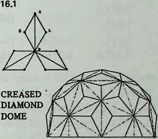
By building the entire dome in this way we can eliminate the strutted frame entirely and allow the joined edges of diamonds and the creases down the centers of the diamonds to take its place. Such a dome has in effect a single circumsphere, passing through all vertices, but two different in spheres, the and the 2v, the difference between the radii of the latter is the virtual thickness we have conferred.
The diamond geometry is independent of dual radii. It was first worked out in the early 1950s, for a structure erected in Woods Hole, Massachusetts, and is interesting because it permits a structure with two diamond diagonals but only one edge length.[11]
Diagram 16.2 shows how. We want to make 0,0/1,0 equal to 1,0/2,1. We commence by noting that if 2,1 (the centroid of the icosa face) has coordinates 0, 0 while 1,0 has coordinates then the distance 0,0/1,0 will be (by Equation 9.2):
and the distance 1,0/2,1 will be: $$\sqrt{2 - 2 (\cos \Theta \cos \Theta_{1}+ \cos \phi \sin \Theta_{1}\sin \Theta)}.$$ 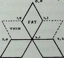
From the Class I table (Chapter 20) we learn that the coordinates of 2,1, the centroid of the icosa face triangle, are 36, 37.3773681. We insert these values for 0 and 0, equate the two expressions with one another, and solve this equation for , which proves to be .
From this we derive a icosa breakdown using only 3 chord factors:
0,0/1,0
1,0/2,1
1,0/1,1
1,0/2,0
0.393411
0.453480
0.313800
(all diamond edges)
(fat-diamond diagonal)
(thin-diamond diagonal)
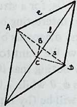
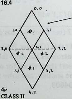
These chord factors are for a dome made in the usual way, out of struts. To make it of creased diamonds, we need two more distances, the long diagonal common to every fat diamond (0,0/2,1) and the long diagonal of every thin diamond (2,1/4,2). These are 0.640852 and 0.713644, respectively.
A little experimenting with cardboard diamonds will show that once the edges are correctly cut, the angles of crease are self-adjusting. For stiffer material, for instance, sheet metal creased in a brake, we would want to know the crease angles in advance. As Diagram 16.3 shows, they are easily calculated: 166.8° for the fat diamond, 142.52° for the thin.
If we make a cardboard model, or even fit just a few cardboard diamonds together, we can easily see that, whereas the material is thin, the geometry of the shell confers virtual thickness, interesting but unnecessary for a frequency this low. The easiest way to extend the principle to higher frequencies where it can be of some use is to work from a Class II breakdown. Diagram 16.4 shows the derivation of the diamonds for a and Diagram 16.5 shows how they fit together. Again, a second breakdown has appeared: the creases outline a Class I. Coordinates need not be tampered with, but simply taken from the Class II table (Chapter 21 or Chapter 23). Again two diamonds suffice.
It should now be clear how higher frequencies would be dealt with. Make a Class II breakdown diagram; mark symmetries (that is, equal chord factors: colored pencils are useful); outline the diamonds; calculate the necessary chord factors, remembering to include the long diagonal of each diamond. If the crease angle is needed, obtain it as shown in Diagram 16.3. The creases will follow a Class I breakdown at half the chosen frequency.
Both of the Class II breakdown methods discussed in this book yield two diamonds at . At higher frequencies Method 3 displays its usual economies, the number of different diamonds being just half the frequency count (four for , eight for ). Method 1 requires six diamonds for and twenty for , the number of different components, as usual, increasing rapidly.
¶ Trussed Frames
The other principal method of lending stiffness to a shell of high frequency (low local curvature) is to use an outer frame and an inner frame and truss them together.
The American Society for Metals (ASM) dome in Cleveland (Popko, figures 69–72) consists of two shells of identical geometry, each Class II, the radius of the inner one 30 inches less than the radius of the outer, joined together at the vertex points by 30-inch radials. How something like this could be designed is obvious: two sets of strut lengths are figured, using the same chord factors but two slightly different radii.
To save weight (and lend grace) numerous struts are omitted, leaving a pattern of hexagons which are then stabilized tensionally, the tension cables replacing the omitted struts (Popko, figure 71, shows connector details).
Or the two shells need not be identical. The Montreal Expo ‘67 dome, a tour de force of design by Fuller and Sadao Inc., in effect trusses a Class I outer grid to a Class II inner grid. As we learned from our discussion of diamonds, both classes can be derived from Class II coordinates by choosing different points to interconnect. Diagram 16.6 shows the principle, using a lower pair of frequencies ( and ). The hexagon pattern is the inner shell, obtained by joining selected Class II vertices. The triangle pattern is the outer shell, obtained by joining vertex pairs as shown. Finally the missing struts in the hex-pattern inner shell are replaced by truss members which rise from the hex corners to meet, six at a time, at the outer shell vertices. The result is an exceedingly rigid space frame, virtually a spherical octet truss.
As an exercise, we may quickly obtain every member length in our example. Let us assume a ratio of 100/95 for the radii of the two shells and select Class II Method 3 for its characteristic economies. We first see which chord factors we need; Diagram 16.7 shows that the hex and pent boundaries use only 3 lengths, b, c, and h. We extract these directly from the table in Chapter 23, and because this shell will have a radius of 0.95 we take 95 percent of the result:
Class II Method 3
(r = 0.95)
1,0/1,1 0.189484
1,0/2,0 0.158653
4,0/4,1 0.160239
We next obtain chord factors for the outer shell’s triangulation, using Equation 9.2 and the coordinates from the table. This shell has a radius of 1, so the chord factors are written down exactly as they come from the calculator. (Just one detail: the strut from 2,1 which crosses the Class II triangle’s edge goes to in the next Class II triangle. This point has the same as 2,1 in the table, but its 0 will be 72° higher instead of 36.) Only four values occur, and if our understanding of Class II Method 3 symmetry was insufficient to tell us this, we should soon find it out by experiment.
4v Class I (r = 1.0)
0,012,1 k 0.275904
2,112,1 I 0.321244
2,113,0 m 0.314751
3,0/5,1 0.264769
2,1 /4,2 is the same as 0,0/2,1 and 3,0/4,2 is the same as 2,1 /3,0; the other symmetries are obvious.
The truss members, finally. We know the spherical coordinates of every pair of points in which we are interested, and the standard formulae will give us the distance between them, regardless of the fact that they are not located on a common sphere. One point of each pair is located on an inner shell, one point on an outer. We simply use Equation 9.1 and both radii, 1.0 and 0.95. Of the eight member lengths in the Method 3 breakdown, hex and pent edges have already accounted for three; the trusses correspond to the other five.
truss members = 1, r2 = 0.95)
| ,0/1,0 | ||
| ,0/2,! | ||
| ,0/3,0 | ||
| ,0/3,1 | ||
| ,0/4,0 |
These are used exactly like chord factors: we multiply by the radius of the outer shell to get the actual lengths of truss members. The lengths of inside shell members are also obtained by using the outside shell radius, the correction having been already built into the chord factors.
This very intricate two-shell trussed domical space frame uses members of just twelve different lengths. It’s not a backyard project. The hubs would need careful study. Each hub on the outer shell receives twelve members, each hub on the inner shell six. Hub design would need angles which Chapter 17 tells how to obtain.
¶ About Angles
A geodesic structure contains three main kinds of angular relationships about which we may need information: (1) Axial. This is the angle between a strut and the sightline from its end to system center. It is a function of strut length and local radius. If the system is spherical (all radii = 1) each strut length has its unique axial angle, the same at either end. If the system is non-spherical, varying radii may produce different axial angles at the two ends of a strut, and still different ones for the same strut length at different positions in the system. (2) Face. The comer angles of a face triangle. (3) Dihedral. The angles between adjacent triangular planes.
What angles we may want to know will depend on the method of construction we envisage. The builder of a wooden frame needs axial angles to know how to cut his struts where their ends meet. Hub design requires axial and face angles. To assemble pieces of paneling into a skin with snugly butted edges, we need dihedral angles. (The crease angle we encountered in our discussion of diamond panels was a species of dihedral, easy to calculate because the diamond was highly symmetrical.) Detailed information follows.
¶ Axial Angles
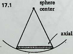
Diagram 17.1 shows that when the system is spherical the axial angles are at the base of an isosceles triangle whose apex is the central angle subtended by a strut. So each axial angle is 1/2(180° - central angle). And we can derive the central angle from the chord factor, which by definition is twice the sine of half the central angle. Combining these observations, we find that for a spherical system,
If the system is non-spherical, we need, in addition to the strut’s chord factor, the radii at its two ends, which will be in our work sheets because obtained them when we were calculating the chord factor in the first place. Diagram 17.2 shows the triangle we are now solving. If the strut is , its chord factor a, and the radii at ends and are and , respectively, then,
After which, more simply,
¶ Face Angles
From the freshman trig text: given the three sides of a triangle, to find its three angles. The sides are simply the chord factors of the struts that bound a face. In Diagram 17.3, if the triangle has sides and , then
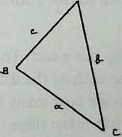
We can use this result to find the next angle more quickly:
And the last one more quickly still:
¶ Dihedral Angles
The existence of an elegant procedure seems plausible, but so long as it continues to be elusive, we can rely on trigonometric brute force. Diagram 17.4 shows what we are trying to accomplish. We want the dihedral angle between triangle and triangle . A “normal plane” passes through their common edge and the system center, and it is not too difficult to obtain the angle at which each triangle meets this plane. We can then obtain the dihedral by adding these two angles together.
Start with triangle ABC. We know its three sides (chord factors) and the radii of its three vertices (= 1 for spheres). We know the face angle at (or know how to obtain itsee above). We also know or can obtain the axial angle at B. A perpendicular to the side marks off segment , the length of which will be cos Bf (Bf being the face angle). In the triangle we now know 2 sides, and the radius BO; the angle included between them will be the axial angle Ba, which we also know how to obtain. So we can find side , which is also a side of triangle AXO. The sideAY of this triangle is sin By, and its third side is the radius at A So we can calculate what we want to find, the angle AXO. Using data for triangle , we repeat the process to obtain angle , and add these results. The sum is the dihedral. When all radii = 1 (the spherical case) this procedure shakes down to:
This method is messy but exact. To see how often we must go through it, we examine each of the different strut lengths in a breakdown diagram to see how many different pairs of triangles meet across it. Each strut is the ridge of a dihedral angle, and if our system is spherical the dihedrals along identical boundaries between like pairs of triangles will be identical.
Diagram 17.5 shows all the triangle types in the rotated and truncated octahedron we designed in Chapter 14. Its forty-five triangles are of just four types, the ones that group in hexagons, the ones that group in squares, and the two special ones produced by the truncation process. Of the five different strut lengths, occurs on four kinds of boundaries: between and ; between and ; between and ; between and . Length occurs only between and ; length . Length never occurs between pairs of triangles, only between a triangle and the floor (more about this later). Length is found only between and .
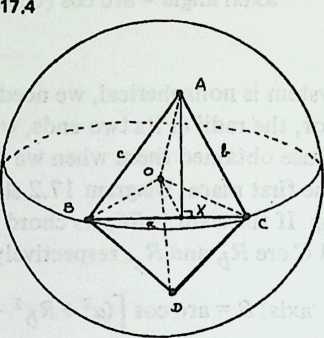
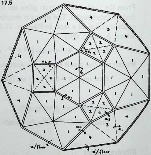
So this structure contains just seven dihedral angles, not an excessive number to figure if our method of construction should require them. The four triangles will have a total of twelve face angles, and the five strut lengths will have five axial angles. The complete set is tabulated herewith (Table 17.1) for the reader to check as an exercise.
Table 17.1 3v Octa, Rotated and Truncated
(complete angular data)
| Face | ||||
| Face | ||||
| Dihedral all | ||||
| Dihedral a 1 2 | ||||
| Dihedral a 2 3 | ||||
| Al: | Face | Dihedral a 1 4 | ||
| Face | Dihedral 1 1 | |||
| A2: | Face | Dihedral c 2 2 | ||
| Face | Dihedral 3 4 | |||
| Face | ||||
| Face | Wall/floor, | |||
| A4: | Face | Wall/floor, |
Note: “Face ab” means the face angle between struts a and b. “Dihedral a 1 1” means the dihedral angle between two #1 triangles where they meet along side a. For triangle numbering see Diagram 17.5.
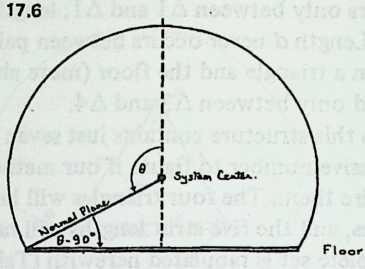 A word on the meeting of panel with floor (along strut and sometimes strut in this example). This constitutes a special kind of dihedral angle. Should we want to know it, we divide the problem as before into two parts. We use Equation 1 l.l to find the angle between the triangular panel and a “normal plane” through system center. If we are dealing with a hemisphere, the floor occupies this plane and the calculation is finished. If we are not, we need also the angle between the normal plane and the floor. Diagram 17.6 shows that this follows directly from the 0 of the truncation plane: it is simply 6 - 90°. We add this to what Equation 17.7 gave us; the result will be the angle between panel and floor, as viewed (like all dihedral angles) from inside the structurean acute angle if the structure is less than a hemisphere, obtuse if it is more. (The acute-obtuse correction is supplied automatically by the fact that 6 - 90° will be negative if the structure is less than a hemisphere, so the net effect of adding it will be to diminish the dihedral.) In our rotated/truncated octa example, the truncation plane 0 is 104.963218°, so we add 14.963218° to the angle between bottom triangles and the normal plane, giving us dihedral angles of slightly more than 90°. At 14° below the equator, a octa structure is just commencing to display outward curvature.
Nonspherical dihedrals remain to be considered. It is a comfort to know that they are rarely needed. They are tedious to arrive at, both because varying radii complicate the expressions, and because there are apt to be so many different ones. Anyone engaged in the design of a high-frequency nonspherical geodesic structure presumably has a budget sufficient to rent computer time if dihedral angles are needed. What will need to be gotten through the computer’s head is a procedure essentially like that which yielded Equation 17.7, complicated however by the fact that the three radii of a triangle’s vertices are no longer equal. The discussion that accompanied Diagram 17.4 may be reread with this fact in mind.
By staying calm we arrive at the following procedure:
-
Obtain the axial angle Ba with Equation 17.2
-
Obtain length as follows:
OX =Vc^{2}\cos^{2}B+jR^{2}-2c \cos BR \cos B_{a}.\label{eq:17.8} -
Obtain Angle as follows: $$angle AXO =\arccos (c{2}\sinBy + OX^{2}- R_{a}^{2}/2c OX \sin By).\label{eq:17.9}$$
Repeat with the second triangle, and add.
¶ Data
¶ Class I Octahedral Coordinates
Eight frequenciesare here combined in three tables. Pick the vertex labels for the frequency you are using out of the proper column at the left, and find the and coordinates at the right.
Each table covers one octahedron face whose comers are 0,0; 0,90; 90,90. For spheres use only the symmetry triangle (Diagram 12.1). For ellipsoids of revolution (one cross-section circular) use the left half of the triangle. When both floorplans and rooflines are non-circular use the entire triangle.
If plans for coordinate rotation should require data on part of the #2 triangle (down-pointing below the equator) simply repeat values from the #1 triangle and add 90 to values.
A peculiar symmetry of the octahedron permits all coordinates to be written in two notations: arctan and decimal degrees. “Arctan 3” (three keystrokes) is quicker to key on the calculator than “71.5650512” (ten keystrokes) and the entered number is identical. With expressions like “” the saving in keystrokes vanishes but the likelihood of error remains less, symbols on the keyboard being less easily confused than digits. But use the decimal forms if you prefer.
Coordinates were generated by an HP-65 program using Equations 12.1 and 12.2.
OCTAHEDRON CLASS I COORDINATES: Frequencies 12, 6, 3
| 3v 6v 12v | V | e |
| ,0 0,0 0,0 |
|
|
|
|
arctan 1/11 5.1944289 arctan 1/11 5.1944289 |
1,0 2,0
1,1 2,2 |
arctan 1 45.0000000
|
arctan 1/5 11.3099325 arctan 72/10 8.0494670 arctan 1/5 11.3099325 |
|
arctan 1/2 26.5650512 arctan 2 63.4349488
|
arctan 1/3 18.4349488 arctan 75/81 13-9527364 arctan 75/81 13.9527364 arctan 1/3 18.4349488 |
1,0 2,0 4,0
2,1 4,2
1,1 2,2 4,4 |
arctan 1/3 18.4349488 arctan 1 45.0000000 arctan 3 71.5650512
|
arctan 1/2 26.5650512 arctan 75/32 21.5681294 arctan 71/8 19.4712206 arctan 75/32 21.5681294 arctan 1/2 26.5650512 |
|
arctan 1/H 14.0362435 arctan 2/3 33.6900675 arctan 3/2 56.3099324 arctan 4 75.9637566
|
arctan 5/7 35.5376778 arctan 717/49 30.4987270 arctan 713/49 27.2520337 arctan 713/49 27.2520337 arctan 717/49 30.4987270 arctan 5/7 35.5376778 |
3,0 6,0
3,1 6,2
3,2 6,4
3,3 6,6 |
arctan 1/5 11.3099325 arctan 1/2 26.5650512 arctan 1 45.0000000 arctan 2 63.4349488 arctan 5 78.6900675
|
arctan 1 45.0000000 arctan 713/18 40.3591005 arctan 75/9 36.6992252 arctan 71/2 35.2643897 arctan 75/9 36.6992252 arctan 713/18 40.3591005 arctan 1 45.0000000 |
|
arctan 1/6 9.4623222 arctan 2/5 21.8014095 arctan 3/4 36.8698977 arctan 4/3 53.1301024 arctan 5/2 68.1985905 arctan 6 80.5376778
|
arctan 7/5 54.4623222 arctan 737/25 50.5799684 arctan 729/25 47j1240113 arctan 1 45.0000000 arctan 1 45.0000000 arctan 729/25 47.1240113 arctan 737/25 50.5799684 arctan 7/5 54.4623222 |
2,0 4,0 8,0
4,1 8,2
|
arctan 1/7 8.1301024 arctan 1/3 18.4349488 arctan 3/5 30.9637565 |
arctan 2 63.4349488 arctan 725/8 60.5037915 arctan 75/2 57.6884668 Aretan 717/8 55.5500980 |
3v 6v 12v 2,1 4,2 8,4
4,3 8,6
2,2 4,4 8,8 |
V arctan 1 45.0000000 arctan 5/3 59.0362435 arctan 3 71.5650512 arctan 7 81.8698977
|
arctan /2 54.7356103 arctan /17/8 55.5500980 arctan /5/2 57.6884668 arctan /25/8 60.5037915 arctan 2 63.4349488 |
|
arctan 1/8 7-1250164 arctan 2/7 15-9453959 arctan 1/2 26.5650512 arctan 4/5 38.6598083 arctan 5/4 51-3401917 arctan 2 63.4349488 arctan 3.5 74.0546041 arctan 8 82.8749836
|
arctan 3 71.5650512 arctan /65/9 69.5895545 arctan /53/9 67.6043377 arctan /5 65.9051575 arctan /41/9 64.8959097 arctan /41/9 64.8959097 arctan /5 65.9051575 arctan /53/9 67.6043377 arctan /65/9 69.5895545 arctan 3 71.5650512 |
5,0 10,0
5,1 10,2
5,2 10,4
5,3 10,6
5,4 10,8
5,5 10,10 |
arctan 1/9 6.3401918 arctan 1/4 14.0362435 arctan 3/7 23.1985905 arctan 2/3 33.6900675 arctan 1 45.0000000 arctan 3/2 56.3099325 arctan 7/3 66.8014095 arctan 4 75.9637566 arctan 9 83-6598082
|
arctan 5_ 78.6900675 arctan /41/2 77.5454236 arctan /17~ 76.3669778 arctan /29/2 75.2856464 arctan /13 74.4986405 arctan /25/2 74.2068310 arctan /TJ 74.4986405 arctan /29/2 75.2856464 arctan /I? 76.3669778 arctan /41/2 77.5454236 arctan 5 78.6900675 |
|
arctan 1/10 5.7105931 arctan 2/9 12.5288077 arctan 3/8 20.5560452 arctan 4/7 29.7448813 arctan 5/6 39.8055711 arctan 6/5 50.1944289 arctan 7/4 60.2551187 arctan 8/3 69.4439548 arctan 4.5 77.4711923 arctan 10 84.2894069
|
arctan 11 84.8055711 arctan /101 84.3175615 arctan /E5 83.8096005 arctan /73 83.3244079 arctan /b5 82.9294449 arctan /51 82.7037247 arctan /61 82.7037247 arctan /&5 82.9294449 arctan /73 83.3244079 arctan /85 83.8096005 arctan /101 84.3175615 arctan 11 84.8055711 |
3,0 6,0 12,0
6,1 12,2
3,1 6,2 12*4
6,3 12,6
3,2 6,4 12,8
|
arctan 1/11 5.1944289 arctan 1/5 11.3099325 arctan 1/3 18.4349488 arctan 1/2 26.5650512 arctan 5/7 35.5376778 arctan 1 45.0000000 arctan 7/5 54.4623222 arctan 2 63.4349488 arctan 3 71-5650512 |
|
| ,5 12,10 | arctan 5 78.6900675 |
|
|
arctan 11 84.8055711 |
|
| ,3 6,6 12,12 |
|
OCTAHEDRON CLASS I COORDINATES: Frequencies 8, 4, 2
| \ | 4v | 8v | ||||
| ,0 | ,0 | ,0 | ||||
| ,0 | arctan 1/7 | |||||
| ,1 | arctan 1/7 | |||||
| ,0 | ,0 | arctan 1/3 | ||||
| ,1 | arctan 1 | arctan /1/18 | ||||
| ,1 | ,2 | arctan 1/3 | ||||
| ,0 | arctan 3/5 | |||||
| ,1 | arctan 1/2 | arctan /1/5 | ||||
| ,2 | arctan 2 | arctan /1/5 | ||||
| ,3 | arctan 3/5 | |||||
| ,0 | ,0 | ,0 | arctan 1 | |||
| M | arctan 1/3 | arctan /5/8 | ||||
| ,1 | ,2 | arctan 1 | arctan /1/2 | -2643897 | ||
| arctan 3 | arctan /5/8 | |||||
| ,1 | ,2 | ,4 | arctan 1 | |||
| ,0 | arctan 5/3 | |||||
| ,1 | arctan 1/4 | arctan /17/9 | ||||
| ,2 | arctan 2/3 | arctan /13/9 | ||||
| ,3 | arctan 3/2 | arctan /13/9 | ||||
| ,4 | arctan 4 | arctan /17/9 | ||||
| ,5 | arctan 5/3 | |||||
| ,0 | ,0 | arctan 3 | ||||
| ,1 | arctan 1/5 | arctan /13/2 | ||||
| ,1 | ,2 | arctan 1/2 | arctan /T | |||
| ,3 | arctan 1 | arctan /g/2 | ||||
| ,2 | ,4 | arctan 2 | arctan /5 | |||
| ,5 | arctan 5 | arctan /13/2 | ||||
| ,3 | ,6 | arctan 3 | ||||
| ,0 | arctan 7 | |||||
| ,1 | arctan 1/6 | arctan /37 | ||||
| ,2 | arctan 2/5 | arctan /29 | ||||
| ,3 | arctan 3/4 | arctan 5 | ||||
| ,4 | arctan 4/3 | arctan 5 | ||||
| ,5 | arctan 5/2 | arctan /29 | ||||
| ,6 | arctan 6 | arctan /37 | ||||
| ,7 | arctan 7 |
| 2v 8\> | V | |
o co o o CXJ |
|
|
|
arctan 1/7 8.1301024 |
|
| ,1 8,2 | arctan 1/3 18.4349488 |
|
|
arctan 3/5 30.9637565 |
|
| ,1 4,2 8,4 | arctan 1 45.0000000 |
|
|
arctan 5/3 59.0362435 |
|
| ,3 8,6 | arctan 3 71-5650512 |
|
|
arctan 7 81.8698976 |
|
| ,2 4,4 8,8 |
|
|
OCTAHEDRON CLASS I COORDINATES: Frequencies 10, 5, 2
| 2v | 5v | lOv | |||||
| ,0 | ,0 | ,0 | |||||
| 6.3401917 | |||||||
,0 1,1 |
,0 2,1 2,2 |
arctan 1 | 45.0000000 90.0000000 |
arctan arctan arctan |
1/4 /1/32 1/4 |
10.0249879 14.0362435 |
|
arctan 1/2 arctan 2 |
26.5650512 63.4349488 90.0000000 |
17.7154723 17.7154723 23.1985905 |
|||||
,0 2,1 2,2 |
,0 4,1 4,2 4,3 4,4 |
arctan 1/3 arctan 1 arctan 3 |
18.4349488 45.0000000 71.5650512 90.0000000 |
arctan arctan arctan arctan arctan |
2/3 ✓5/18 /2?9 ✓5/18 2/3 |
27.7913057 25.2394018 27.7913057 33.6900675 |
|
,0 1,1 |
,0 5,1 5,2 5,3 5,4 5,5 |
arctan 1/4 arctan 2/3 arctan 3/2 arctan 4 |
14.0362435 33.6900675 56.3099325 75.9637566 90.0000000 |
arctan arctan arctan arctan arctan arctan |
✓17/25 ✓13/25 ✓13/25 ✓17/25 1 |
39.5097123 35.7957599 35.7957599 39.5097123 45.0000000 |
|
,0 3,1 3,2 3,3 |
,0 6,1 6,2 6,3 6,4 6,5 6,6 |
arctan 1/5 arctan 1/2 arctan 1 arctan 2 arctan 5 |
11.3099325 26.5650512 45.0000000 63.4349488 78.6900675 90.0000000 |
arctan arctan arctan arctan arctan arctan arctan |
/2 ✓13/8 ✓574 ✓97F ✓57T ✓13/8 3/2 |
51.8870735 48.1896851 46.6861434 48.1896851 51.8870735 56.3099325 |
|
,0 7,1 |
arctan 1/6 | 9.4623222 | arctan arctan |
/3 ✓37/9 |
63.7476249 |
| 2v | 5v | lOv | ||||||
| ,2 | arctan | /5 | arctan | /29/9 | ||||
| ,3 | arctan | /4 | arctan | <25/9 | ||||
| ,4 | arctan | /3 | arctan | /25/9 | ||||
| ,5 | arctan | /2 | arctan | <29/9 | ||||
| ,6 | arctan | arctan | ✓37/9 | |||||
| ,7 | arctan | /3 | ||||||
| ,0 | ,0 | arctan | ||||||
| ,1 | arctan | /7 | arctan | /25/2 | ||||
| ,1 | ,2 | arctan | /3 | arctan | /10 | |||
| ,3 | arctan | /5 | arctan | ✓17/2 | ||||
| ,2 | ,4 | arctan | arctan | /S’ | ||||
| ,5 | arctan | /3 | arctan | ✓17/2 | ||||
| ,3 | ,6 | arctan | arctan | /io | ||||
| ,7 | arctan | arctan | /25/2 | |||||
| ,8 | arctan | |||||||
| ,0 | arctan | |||||||
| ,1 | arctan | /8 | arctan | |||||
| ,2 | arctan | /7 | arctan | |||||
| ,3 | arctan | /2 | arctan | |||||
| ,4 | arctan | /5 | arctan | Al | ||||
| ,5 | arctan | /4 | arctan | AT | ||||
| ,6 | arctan | arctan | ||||||
| ,7 | arctan | /2 | arctan | |||||
| ,8 | arctan | arctan | /U5 | |||||
| ,9 | arctan | |||||||
| ,0 | ,0 | ,0 | ||||||
| ,1 | arctan | /9 | ||||||
| ,1 | ,2 | arctan | /4 | |||||
| ,3 | arctan | /7 | ||||||
| ,2 | ,4 | arctan | /3 | |||||
| ,1 | ,5 | arctan | ||||||
| ,3 | ,6 | arctan | /2 | |||||
| ,7 | arctan | /3 | ||||||
| ,4 | ,8 | arctan | ||||||
| ,9 | arctan | |||||||
| ,2 | ,5 | ,10 |
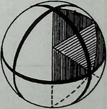
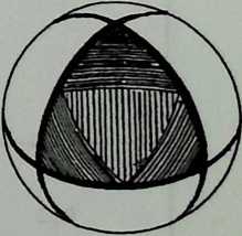
Sphere covered with
Class II triangles.
Two Class II triangles
and halves of two others … rotated 45° = Octa face.
¶ Class II Method 1 Octahedral Coordinates
Two tables provide Class II Method 1 information for the octa breakdown in the following array of frequencies: . (The reader will remember that all Class II frequencies are even.)
For the arctan notation see the introductory page for Class I octa coordinates.
To simplify elliptical breakdowns, data for an area equivalent to the entire octa face are given. This consists of the Class II triangle, its downward-pointing reflection below it, and portions to the left Spherical Octa face and right of the latter: see Diagram 19.1. For spheres use only the symmetry triangle (Diagrams 12.4 and 19.2). For ellipsoids of revolution (one cross-section circular) use the left half of the face. When both roofline and floorplan are non-arcular use the entire face.
Class II triangle coordinates were obtained by an HP-65 program V using Equations 12.1 and 12.3. A second program then obtained the remaining points by successive rotations using Equations 14.1, 14.2.
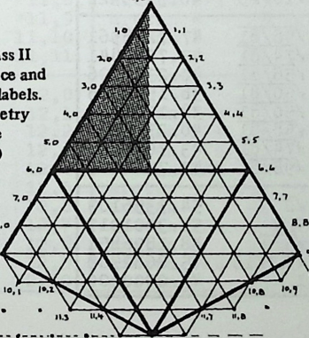
| 4v 8v 16v |
|
e |
| ,0 0,0 0,0 |
|
|
|
|
arctan 72/225 5-3859771 arctan /2/225 5.3859771 |
O rd CXJ c * CXJ CXJ CXJ O rd rd rd |
arctan 1 45.0000000
|
arctan /2/49 11.4217537 arctan 71/49 8.1301024 arctan /2/49 11.4217537 |
|
arctan 1/2 26.5650512 arctan 2 63.4349488
|
arctan 718/169 18.0744548 arctan 710/169 13.6717877 arctan 710/169 13.6717877 arctan 718/169 18.0744548 |
o rd cxj cn-=r O rd CXJ CXJ CXJ CXJ O rd rd rd |
arctan 1/3 18.4349488 arctan 1 45.0000000 arctan 3 71.5650512
|
arctan 72/9 25.2394018 arctan 75/36 20.4393176 arctan 1/3 18.4349488 arctan 75/36 20.4393176 arctan 72/9 25.2394018 |
|
arctan 1/4 14.0362435 arctan 2/3 33.6900675 arctan 3/2 56.3099325 arctan 4 75.9637566
|
arctan 750/121 32.7338966 arctan 734/121 27.9274604 arctan 726/121 24.8699503 arctan 726/121 24.8699503 arctan 734/121 27-9274604 arctan 750/121 32.7338966 |
3,0 6,0
3,1 6,2
3,2 6,4
3,3 6,6 |
arctan 1/5 11.3099325 arctan 1/2 26.5650512 arctan 1 45.0000000 arctan 2 63.4349488 arctan 5 78.6900675
|
arctan /18/25 40.3155422 arctan 713/25 35.7957599 arctan 7275 32.3115332 arctan 3/5 30.9637565 arctan /2/5 32.3115332 arctan 713/25 35.7957599 arctan 718/25 40.3155422 |
|
arctan 1/6 9.4623222 arctan 2/5 21.8014095 arctan 3/4 36.8698976 arctan 4/3 53.1301024 arctan 5/2 68.1985905 arctan 6 80.5376778
|
arctan 798/81 47.7248561 arctan 774/81 43.7057841 arctan /58/8I 40.2377996 arctan 750/81 38.1558065 arctan 750/81 38.1558065 arctan /58/81 40.2377996 arctan 774/81 43.7057841 arctan 798/81 47.7248561 |
2,0 4,0 8,0
4,1 8,2
2,1 4,2 8,4 |
arctan 1/7 8.1301024 arctan 1/3 18.4349488 arctan 3?5 30.9637565 arctan 1 45.0000000 |
arctan /2 54.7356103 arctan 5/4 51.3401917 arctan 7577 48.1896851 arctan ✓ 17/16 45.8682508 arctan 1 45.0000000 |
| 4v | 8v | 16v | ||||||
| 2,2 | ,3 4,4 |
,5 8,6 8,7 8,8 |
arctan arctan arctan |
/3 3 7 |
71.5650512 81.8698976 90.0000000 |
arctan arctan ar ct an arctan |
✓17/16 /5X 5/4 /2 |
48.1896851 51.3401917 54.7356103 |
| ,0 | arctan | <32/9 | ||||||
| ,1 | arctan | /8 | arctan | <130/49 | ||||
| ,2 | arctan | /7 | arctan | ✓106/49 | ||||
| ,3 | arctan | /2 | arctan | ✓90/49 | ||||
| ,4 | arctan | /5 | arctan | ✓82/49 | ||||
| ,5 | arctan | /4 | arctan | ✓82/49 | ||||
| ,6 | arctan | arctan | ✓90/69 | |||||
| ,7 | arctan | /2 | arctan | ✓106/49 | ||||
| ,8 | arctan | arctan | ✓130/49 | |||||
| ,9 | arctan | ✓32/9 | ||||||
| ,0 | ,0 | arotan | /S | |||||
| ,1 | arctan | /8 | arctan | <26/5 | ||||
| ,1 | ,2 | arctan | /4 | arctan | ✓34/9 | |||
| ,3 | arctan | /7 | arctan | ✓29/9 | ||||
| ,2 | ,4 | arctan | /3 | arctan | ✓26/9 | |||
| ,5 | arctan | arctan | ✓25/9 | |||||
| ,3 | ,6 | arctan | /2 | arctan | ✓26/9 | |||
| ,7 | arctan | /3 | arctan | ✓29/9 | ||||
| ,4 | ,8 | arctan | arctan | ✓34/9 | ||||
| ,9 | arctan | arctan | ✓26/5 | |||||
| ,5 | ,10 | arctan | /b* | |||||
| ,0 | arctan | ✓32 | ||||||
| ,1 | arctan | /8 | arctan | ✓130/9 | ||||
| ,2 | arctan | /4 | arctan | ✓17/2 | ||||
| ,3 | arctan | /8 | arctan | ✓146/25 | ||||
| ,4 | arctan | /7 | arctan | ✓26/5 | ||||
| ,5 | arctan | /6 | arctan | ✓122/25 | ||||
| ,6 | arctan | /5 | arctan | ✓122/25 | ||||
| ,7 | arctan | /4 | arctan | ✓26/5 | ||||
| ,8 | arctan | /3 | arctan | ✓146/25 | ||||
| ■11,9 | arctan | arctan | <17/2 | |||||
| ,10 | arctan | arctan | ✓130/9 | |||||
| ,11 | arctan | /32 | ||||||
| ,0 | ,0 | ,0 | ||||||
| ,1 | arctan | /8 | arctan | /I30 | ||||
| ,1 | ,2 | arctan | /4 | arctan | ✓34 | |||
| ,3 | arctan | /8 | arctan | ✓146/9 | ||||
| ,1 | ,2 | ,4 | arctan | /2 | arctan | ✓10 | ||
| ,5 | arctan | /7 | arctan | ✓37/4 | ||||
| ,3 | ,6 | arctan | arctan | |||||
| ,7 | arctan | /5 | arctan | ✓37/4 | ||||
| ,2 | ,4 | ,8 | arctan | arctan | /io | |||
| ,9 | arctan | /3 | arctan | ✓146/9 | ||||
| ,5 | ,10 | arctan | arctan | ✓34 |
| 4v 8v 16v | ||
3,3 6,6 12,12 |
arctan 8 82.8749836
|
arctan 7130 84.9876536
|
|
arctan 1/8 7-1250163 arctan 1/4 14.0362435 arctan 3/8 20-5560452 arctan 1/2 26.5650512 arctan 5/8 32.0053832 arctan 6/7 40.6012947 arctan 7/6 49-3987054 arctan 8/5 57-9946168 arctan 2 63.4349488 arctan 8/3 69-4439548 arctan 4 75-9637566 arctan 8 82.8749836 |
arctan -7130 95.0123464
arctan 71T6 85.2689493 arctan /To 81.0151231 arctan 7178/9 77-3272785 arctan 7170/9 77-0423654 arctan 7170/9 77-0423654 arctan 7178/9 77-3272785 arctan 75o 81.0151231 arctan 7146 85.2689493
arctan -7130 95.0123464 |
7,2 14,4
7,3 14,6
7,4 14,8
7,5 14,10
|
arctan 3/8 20.5560452 arctan 1/2 26.5650512 arctan 5/8 32.0053832 arctan 3/4 36.8698976 arctan 1 45-0000000 arctan 4/3 53.1301024 arctan 8/5 57-9946168 arctan 2 63.4349488 arctan 8/3 69-4439548 |
arctan -7146 94.7310506
arctan TITS’ 85.7135149 arctan /50 81.9505330 arctan 7 81.8698976 arctan 750 81.9505330 arctan 7178 85.7135149
arctan -TITS’ 94.7310506 |
|
arctan 5/8 32.0053832 arctan 3/4 36.8698976 arctan 7/8 41.1859252 arctan 8/7 48.8140748 arctan 4/3 53.1301024 arctan 8/5 57.9946168 |
arctan -7178 94.2864851
arctan /22T 86.1943478 arctan TITS’ 86.1943478
arctan -7178 94.2864851 |
4,2 8,4 16,8
|
arctan 7/8 41.1859252 arctan 1 45.0000000 arctan 8/7 48.8140748 |
arctan -TUT 93.8056521
arctan -TITS’ 93-8056521 |
| 6v | 12v | |||||
| ,0 | ,0 | |||||
| ,0 | arctan /2/121 | |||||
| ,1 | arctan /2/121 | |||||
| ,0 | ,0 | arctan /2/25 | ||||
| ,1 | arctan | arctan 1/5 | ||||
| ,1 | ,2 | arctan /2/25 | ||||
| ,0 | arctan Z2/9 | |||||
| ,1 | arctan | /2 | arctan /10/81 | |||
| ,2 | arctan | arctan /10/81 | ||||
| ,3 | arctan /2/9 | |||||
| ,0 | ,0 | arctan /1/2 | ||||
| ,1 | arctan | /3 | arctan /5/16 | |||
| ,1 | ,2 | arctan | arctan 1/2 | |||
| ,3 | ar ct an | arctan /5/16 | ||||
| ,2 | ,4 | arctan /1/2 | ||||
| ,0 | arctan /50/49 | |||||
| ,1 | arctan | /4 | arctan /§4/49 | |||
| ,2 | arctan | /3 | arctan /26/49 | |||
| ,3 | arctan | /2 | arctan /26/49 | |||
| ,4 | arctan | ar’ctan /34/49 | ||||
| ,5 | arctan /5O/49 | |||||
| ,0 | ,0 | arctan /T | ||||
| ,1 | arctan | /5 | arctan /13/9 | |||
| ,1 | ,2 | arctan | /2 | arctan /10/9 | ||
| ,3 | arctan | arctan 1 | ||||
| ,2 | ,4 | arctan | arctan /10/9 | |||
| ,5 | arctan | arctan /13/9 | ||||
| ,3 | ,6 | arctan /2 | ||||
| ,0 | arctan /9/2 | |||||
| ,1 | arctan | /6 | arctan Z74/25 | |||
| ,2 | arctan | /5 | arctan /8/25 | |||
| ,3 | arctan | /4 | arctan /2 | |||
| ,4 | arctan | /3 | arctan /2 | |||
| ,5 | arctan | /2 | arctan 758/25 | |||
| ,6 | arctan | arctan /74/25 | ||||
| ,7 | arctan 79/2 | |||||
| ,0 | ,0 | arctan /18 | ||||
| ,1 | arctan | /6 | arctan 72.4/9 | |||
| ,1 | ,2 | arctan | /3 | arctan 75 | ||
| ,3 | arctan | /5 | arctan 717/4 | |||
| ,2 | ,4 | arctan | arctan 2 | |||
| ,5 | arctan | /3 | arctan 717/4 |
| 6v 12v |
|
|
,3 8,6 8,7 4,4 8,-8 |
arctan 3 71.5650512 arctan 6 80.5376778
|
arctan 65.9051575 arctan /74/9 70.7741443 arctan /18 76.7373240 |
,0 9,1 9,2 9,3 9,4 9,5 9,6 9,7 9,8 9,9 |
arctan 1/6 9.4623222 arctan 1/3 18.4349488 arctan 1/2 26.5650512 arctan 4/5 38.6598083 arctan 5/4 51-3401917 arctan 2 63.4349488 arctan 3 71-5650512 arctan 6 80.5376778
|
arctan /jjT 83.3692622 arctan /20 77.3956173 arctan /10 72.4515994 arctan /82/9 71.6702463 arctan /82/9 71.6702463 arctan /10 72.4515994 arctan /20 77-3956173 arctan /T 83.3692622
|
,1 5,1 10,2 10,3 5,2 10,4 10,5 5,3 10,6 10,7 5,4 10,8 10,9 |
arctan 1/6 9.4623222 arctan 1/3 18.4349488 arctan 1/2 26.5650512 arctan 2/3 33-6900675 arctan 1 45.0000000 arctan 3/2 56.3099325 arctan 2 63.4349488 arctan 3 71.5650512 arctan 6 80.5376778 |
arctan -/TT 96.6307378
arctan /90 83.9827152 arctan /2K 78.9041967 arctan 5 78.6900675 arctan /2 78.9041967 arctan /90 83.9827152
arctan -/T7* 96.6307378 |
,3 11,4 11,5 11,6 11,7 11,8 |
arctan 1/2 26.5650512 arctan 2/3 33.6900675 arctan 5/6 39-8055711 arctan 6/5 50.1944289 arctan 3/2 56.3099325 arctan 2 63.4349488 |
arctan -/90 96.0172849
arctan /122 84.8267875 arctan /122 84.8267875
arctan -/90 96.0172849 |
,5 6,6 12,6 12,7 |
arctan 5/6 39.8055711 arctan 1 45.0000000 arctan 6/5 50.1944289 |
arctan -/122 95.1732124
arctan -/122 95.1732124 |
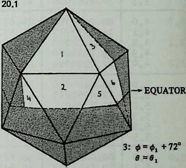
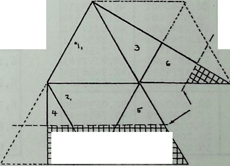
4: 0 = 36
0 = 180° - fl, (when
A #2 is viewed
upside down: see
5:
Fjg. 15.4).
0 = + 36°
fl = same as A #4.
6: </> = 72°+0,
0=0,.
¶ Class I Method 1 Icosahedral Coordinates
Data are given for Class I icosa breakdowns of the following frequencies: . Pick the vertex labels for the fre-quency you are using out of the proper column at the left, and read values from the two columns at the right.
Each table covers two icosa faces: the #1 triangle whose corners are ; 0, ; 72, ; and the downward-pointing #2 triangle beneath it whose comers are 0, ; 72, ; 36, (): see Diagram 12.3. For spheres use only the Symmetry Triangle shown in Diagram 12.2. For ellipsoids of revolution (one cross-section circular) use the left-hand half of both triangles as far down as the proposed truncation plane. For structures with two non-circular cross-sections you need a 90° span of 0 values as well. Diagram 20.1 shows how these can be extrapolated. But such structures have more tractable symmetries if rotated so that an edge, not a vertex, is at the zenith: see Chapter 15.
An HP-65 program using Equations 12.4 through 12.8 generated the values for Triangle #1. A second program using Equations 14.1, 14.2 then generated the Triangle #2 points by rotation.
| 5v lOv | V | |
o o o o |
||
,0 1,1 |
72.0000000 | 5.4084310 |
,0 2,0 2,1 1,1 2,2 |
36.0000000 72.0000000 |
9.2416169 11.3716668 |
,0 3,1 3,2 3,3 |
22.3861776 49.6138225 72.0000000 |
14.9899922 14.9899922 17.8315873 |
m m ro WWW MHO -t Xr UO MHO |
16.0353713 36.0000000 55.9646288 72.0000000 |
21.5724472 20.3856407 21.5724472 24.6710680 |
,0 5,1 5,2 5,3 ‘ 5,4 5,5 |
12.4463843 27.7323015 44.2676986 59.5536157 72.0000000 |
28.6099376 26.8052365 26.8052365 28.6099376 31.7174744 |
,0 6,0 6,1 3,1 6,2 6,3 - 3,2 6,4 6,5 3,3 6,6 |
10.1562304 22.3861776 36.0000000 49.6138225 61.8437696 72.0000000 |
35.8224702 33.7590240 33.0088450 33.7590240 35.8224702 38.7638808 |
,0 7,1 7,2 7,3 7,4 7,5 7,6 7,7 |
8.5725404 18.7046980 30.0743861 41.9256139 53.2953021 63.4274596 72.0000000 |
42.9496334 40.8717741 39.7156131 39.7156131 40.8717741 42.9496334 45.6033616 |
,0 8,0 8,1 4,1 8,2 8,3 4,2 8,4 |
7.4137289 16.0353713 25.7052785 36.0000000 |
49.7664590 47.8353485 46.5286650 46.0642057 |
| 5v lOv | e | |
,5 4,3 8,6 8,7 4,4 8,8 |
55.9646288 64.5862711 72.0000000 |
47.8353485 49.7664590 52.0632820 |
,0 9,1 9,2 9,3 9,4 9,5 9,6 9,7 9,8 9,9 |
6.5297024 14.0192855 22.3861776 31.3846950 40.6153050 49.6138225 57.9807145 65.4702976 72.0000000 |
56.1087309 54.4163133 53.1334950 52.4366973 52.4366973 53.1334950 54.4163133 56.1087309 58.0265179 |
,0 10,0 10,1 5,1 10,2 10,3 5,2 10,4 10,5 5,3 10,6 10,7 5,4 10,8 10,9 5.5 10,10 |
5.8333887 12.4463843 19.7952367 27.7323015 36.0000000 44.2676986 52.2047633 59.5536157 66.1666114 72.0000000 |
61.8829712 60.4665625 59.3117249 58.5495950 58.2825256 58.5495950 59.3117249 60.4665625 61.8829712 63.4349488 |
| ,1 | ||
| ,2 | ||
| ,3 | ||
| ,4 | ||
| ,5 | ||
| ,6 | ||
| ,7 | ||
| ,8 | ||
| ,9 | ||
| ,10 | ||
| ,1 12,2 | ||
| ,3 | ||
| ,2 12,4 | ||
| ,5 | ||
| ,3 12,6 | ||
| ,7 | ||
| ,4 12,8 | ||
| ,9 | ||
| ,5 12,10 |
| 5v 10v | V | e |
,3 13,4 13,5 13,6 13,7 13,8 13,9 13,10 |
17.2607131 24.4947652 32.1184790 39.8815210 47.5052349 54.7392869 61.4051023 |
77.6677097 77.2528359 77.0290522 77.0290522 77.2528359 77.6677097 78.2204432 |
,2 14,4 14,5 7,3 14,6 14,7 7,4 14,8 14,9 7,5 14,10 |
21.1287296 28.4369994 36.0000000 43.5630006 50.8712704 57.7180776 |
83.7703158 83.6117970 83.5562062 83.6117970 83.7703158 84.0101625 |
,5 15,6 15,7 15,8 15,9 |
24.9684505 32.2819224 39.7180776 47.0315495 |
90.0000000 90.0000000 90.0000000 90.0000000 |
| 5v lOv | I . | 6 |
,10 8,3 16,6 16,7 8,4 16,8 16,9 8,5 16,10 |
21.7180776 28.7463723 36.0000000 43.2536277 50.2819224 |
95.9898376 96.1303345 96.1794105 96.1303345 95.9898376 |
,7 17,8 17,9 17,10 |
32.4321744 39.5678256 46.5948977 |
101.9554615 101.9554615 101.7795569 |
,4 18,8 18,9 9,5 18,10 |
36.0000000 42.9684505 |
107.3234344 107.2030468 |
,9 19,10 |
39.4292316 | 112.1491687 |
| ,5 20,10 | II6.5650512 |
| 2v 4v 8v | * | e |
| ,0 0,0 0,0 | ||
|
||
|
||
| ,0 2,0 | ||
|
||
| ,1 2,2 | ||
|
||
|
||
|
||
|
||
| ,0 2,0 4,0 | ||
|
||
| ,1 4,2 | ||
|
||
| ,1 2,2 4,4 | ||
|
||
5,1 |
-0083770 | |
|
||
|
||
|
||
|
||
| ,0 6,0 | ||
|
||
| ,1 6,2 | ||
|
||
| ,2 6,4 | ||
|
||
| ,3 6,6 | ||
|
||
|
||
|
||
|
||
|
||
|
||
|
||
|
| 2v | 4v | 8v | e | |
| ,0 | ,0 | ,0 | ||
| ,1 | ||||
| ,1 | ,2 | |||
| ,3 | ||||
| ,1 | ,2 | ,4 | 36.OOOOOOO | |
| ,5 | ||||
| ,3 | ,6 | |||
| ,7 | ||||
| ,8 |
|
||
|
||
|
||
|
||
|
||
|
||
|
||
|
||
| ,1 10,2 | ||
|
||
| ,2 10,4 | ||
|
||
| ,3 10,6 | ||
|
||
| ,4 10,8 | ||
|
||
|
||
|
||
|
||
|
||
|
||
| ,1 6,2 12,4 | ||
|
||
| ,3 12,6 | ||
|
||
| ,2 6,4 12,8 |
| 2v | 4v | 8v | ||
| ,5 | ||||
| ,6 | ||||
| ,7 | ||||
| ,8 | ||||
| ,3 | ,6 | |||
| ,7 |
| 2v | 4v 7,4 |
8v 14,8 |
V 44.7723551 |
104.5454366 |
,7 15,8 |
40.3045403 | 110.9612167 | ||
| ,2 | ,4 | ,8 |
| 3v | \ | V | |
| ,0 | ,0 | ||
| ,0 | |||
| ,0 | |||
| ,0 | ,0 | ||
| ,1 | |||
| ,1 | ,2 | ||
| ,0 | |||
| ,1 | |||
| ,2 | |||
| ,3 | |||
| ,0 | ,0 | ||
| ,1 | |||
| ,1 | ,2 | ||
| ,3 | |||
| ,2 | ■ 4,4 | ||
| ,0 | |||
| ,1 | |||
| ,2 | |||
| ,3 | |||
| ,4 | .7 | ||
| ,5 | |||
| ,0 | ,0 | ||
| ,1 | |||
| ,1 | ,2 | ||
| ,3 | |||
| ,2 | ,4 | ||
| ,5 | |||
| ,3 | ,6 |
| 3v 6v | V | e |
,1 7,2 7,3 7,4 7,5 7,6 |
16.7344818 29.3546281 42.6453719 55.2655182 66.2221928 |
69.4828700 68.5073635 68.5073635 69.4828700 71.0914502 |
,1 8,2 8,3 4,2 8,4 8,5 4,3 8,6 |
23.3461239 36.0000000 48.6538761 60.1814143 |
79.4443283 79.1876831 79.4443283 80.1168545 |
,3 9,4 9,5 9,6 |
29.8185857 42.1814143 54.0000000 |
90.0000000 90.0000000 90.0000000 |
,2 10,4 10,5 5,3 10,6 |
36.0000000 47.8185858 |
100.0928406 99-8831455 |
,5 11,6 |
41.7778072 | 108.9085499 |
| ,3 12,6 |
Triangle #1
Triangle #2
¶ Class II Method 1 Icosahedral Coordinates
Two tables give Class II Method 1 information for theicosa breakdown of frequencies . (The reader will remember that all Class II frequencies are even.)
The unit of attention is not the icosa face but its Class II tri- angle (see Chapter 10). Five of these triangles are covered in the tables: see Diagram 12.5 and the explanation in Chapter 12. Ellipsoidal structures can thus be computed as far down as an equatorial truncation plane. For spheres we disregard most of the data provided and use only the left half of the top Class II triangle (Diagram 12.4); this would be, for example, the area bounded by 0,0; 4,0; 4,2 in the case shown in Diagram 12.5.
An HP-65 program using Equations 12.4, 12.5, 12.6, 12.7, 12.9 generated the Class II triangle data; a second program then obtained the remaining four triangles by successive rotations using Equations 14.1 and 14.2.
| vi | 12v | e | |
| ,0 | ,0 | ||
| ,0 | |||
| ,1 | |||
| ,0 | ,0 | ||
| ,1 | |||
| ,1 | ,2 | ||
| ,0 | |||
| ,1 | |||
| ,2 | |||
| ,3 | |||
| ,0 | ,0 | ||
| ,1 | |||
| ,1 | ,2 | ||
| ,3 | |||
| ,2 | ,4 | ||
| ,0 | |||
| ,1 | |||
| ,2 | |||
| ,3 | |||
| ,4 | -5536157 | ||
| ,5 | |||
| ,0 | ,0 | ||
| ,1 | |||
| ,1 | ,2 | ||
| ,3 | |||
| ,2 | ,4 | ||
| ,5 | |||
| ,3 | ,6 | -3773681 | |
| ,0 | |||
| ,1 | |||
| ,2 | |||
| ,3 | |||
| ,4 | |||
| ,5 | |||
| ,6 | |||
| ,0 | ,0 | ||
| ,1 | |||
| ,2 | |||
| ,3 | |||
| ,2 | ,4 | ||
| ,5 | |||
| ,3 | ,6 |
| 6v 12v | V | |
| ,0 | ||
| ,1 | ||
| ,2 | ||
| ,3 | ||
| ,4 | ||
| ,5 | ||
| ,6 | ||
| ,0 10,0 | ||
| ,1 | ||
| ,1 10,2 | ||
| ,3 | ||
| ,2 10,4 | ||
| ,5 | ||
| ,3 10,6 | ||
| ,0 | ||
| ,1 | ||
| ,2 | ||
| ,3 | ||
| ,4 | ||
| ,5 | ||
| ,6 | ||
| ,0 12,0 | ||
| ,1 | ||
| ,1 12,2 | ||
| ,3 | ||
| ,2 12,4 | ||
| ,5 | ||
| ,3 12,6 | ||
| ,0 | ||
| ,1 | ||
| ,2 | ||
| ,3 | ||
| ,4 | ||
| ,5 | ||
| ,6 | ||
| ,0 14,0 | ||
| ,1 | ||
| ,1 14,2 | ||
| ,3 | ||
| ,2 14,4 | ||
| ,5 | ||
| ,3 14,6 | ||
| 6v 12v | V | e |
,0 15,1 15,2 15,3 15,4 15,5 15,6 |
5.7778072 11.8185857 18.0000000 24.1814143 30.2221929 36.0000000 |
96.0423546 93.0817398 90.0000000 86.9182604 83.9576455 81.2167695 |
,0 16,0 16,1 8,1 16,2 16,3 8,2 16,4 16,5 8,3 16,6 |
5.7778072 11.8185858 18.0000000 24.1814143 30.2221929 36.0000000 |
102.6366099 99.8831455 96.9043551 93.8073037 90.7158218 87.7468790 |
| 6v 12v | V | e |
| ,0 | ||
| ,1 | ||
| ,2 | ||
| ,3 | ||
| ,4 | ||
| ,5 | ||
| ,6 | ||
| ,0 18,0 | ||
| ,1 | ||
| ,1 18,2 | ||
| ,3 | ||
| ,2 18,4 | ||
| ,5 | ||
| ,3 18,6 |
| \> 4m 8m | > | e |
o o o o a o |
||
|
||
|
,4441473 | |
| ,0 2,0 | ||
|
||
| ,1 2,2 | ||
|
||
|
||
|
||
|
||
o ■=r o CXJ o |
||
|
||
| ,1 4,2 | ||
|
||
| ,1 2,2 4,4 | ||
|
||
|
||
|
||
|
||
|
||
| ,0 6,0 | ||
|
||
| ,1 6,2 | ||
|
||
| ,2 6,4 |
| 2m 4m 8m | V | e |
|
9.7323015 19.9646288 30.0743861 41.9256139 |
64.0653713 59.8480232 56.7273505 56.7273505 |
H cxj cnr oo00 coco co O rd (XI -=r -=r O rd A CXJ CXJ |
.0000000 8.7723551 18.0000000 27.2276449 36.0000000 |
74.4432523 70.0353712 66.3105890 63.4349488 |
|
8.7723551 18.0000000 27.2276449 36.0000000 |
84.3401063 79.7052785 75.4545635 71.8790961 |
5,0 10.0
5,1 10,2
5,2 10,4 |
8.7723551 18.0000000 27.2276449 36.0000000 |
94.5840965 90.0000000 85.4159036 81.2167695 |
|
8.7723551 18.0000000 27.2276449 36.0000000 |
104.5454366 100.2947216 95.6598938 91.0448019 |
3,0 6,0 12,0
6,1.12,2
3,1 6,2 12*4 |
8.7723551 18.0000000 27.2276449 36.0000000 |
113.6894110 109.9646288 105.5567478 100.8123170 |
¶ Tetrahedral Coordinates
Because its breakdowns entail an excessive number of different component lengths, a problem compounded by the high frequencies required to obtain anything acceptably spherical, the tetrahedron is of limited usefulness. Still, investigators may have a use for data. Class II Method 1 is recommended for study. It has orthogonal equators like the octahedron, permitting natural hemispheric truncation, and when so truncated provides large squarish openings at ground level. (0,0 is not at the zenith.)
The designer might also consider omitting some of the shorter struts that clutter the three-way vertices. So long as triangulation is preserved this will do no structural damage and greatly improve the symmetry.
Large families of intersecting equatorseight in the Class I permit numerous zenith locations and overhead symmetries. Two Class I tables provide for the following frequencies: . They cover one tetrahedron face, with comers at .
Two Class II Method 1 tables provide for sixteen, twelve, eight, and six-frequency breakdowns. They cover the Class II triangle with vertices at . See Diagram 22.1 for the location of this triangle; twelve of them make a sphere.
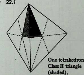
| 3v 6v 12v | V | e |
| ,0 0,0 0,0 | ||
|
||
|
||
| ,0 2,0 | ||
|
||
| ,1 2,2 | ||
|
||
|
||
|
||
|
||
| ,0 2,0 4,0 | ||
|
||
| ,1 4,2 | ||
|
||
| ,1 2,2 4,4 | ||
|
||
|
||
|
||
|
||
|
||
|
||
| ,0 6,0 | ||
|
||
C\J 0 KO 00 |
||
|
||
* KO CM no |
||
|
||
| ,3 6,6 | ||
|
||
|
||
|
||
|
||
|
||
|
||
|
||
|
||
| ,0 4,0 8,0 | ||
|
||
| ,1 8,2 | ||
|
||
| ,1 4,2 8,4 | ||
| 3v 6v 12v | > | |
| ,3 8,6 | ||
|
||
| ,2 4,4 8,8 | ||
|
||
|
||
|
||
|
||
|
||
|
||
|
||
|
||
|
||
|
||
| ,0 10,0 | ||
|
||
| ,1 10,2 | ||
|
||
| ,2 10,4 | ||
|
||
| ,3 10,6 | ||
|
||
| ,4 10,8 | ||
|
||
| ,5 10,10 | ||
|
||
|
||
|
||
|
||
|
||
|
||
|
||
|
||
|
||
|
||
|
||
|
||
| ,0 6,0 12,0 | ||
|
||
| ,1 12,2 | ||
|
||
| ,1 6,2 12,4 | ||
|
||
| ,3 12,6 | ||
|
||
| ,2 6,4 12,8 | ||
| 3v | 6v | 12v | V | e |
| ,5 | ,9 12,10 |
109.1066053 | 114.8398925 |
| 3v | 6v | 12v | V | |
| ,3 | ,6 | ,11 12,12 |
120.0000000 | 109.4712206 |
TETRAHEDRON CLASS I COORDINATES: Frequencies 16, 8, 4
| 4v 8v 16v | V | |
V 0 0 0 0 0 |
||
|
||
|
||
CXI 0 |
||
|
||
| ,1 2,2 | ||
|
||
|
||
|
||
|
||
0 cxj 0 |
||
|
||
| ,1 4,2 | ||
| n 4’3 | ||
| ,1 2,2 4,4 | ||
|
||
|
||
|
||
|
||
|
||
|
||
| ,0 6,0 | ||
|
||
| ,1 6,2 | ||
|
||
| ,2 6,4 | ||
|
||
| ,3 6,6 | ||
|
||
|
||
|
||
|
||
|
||
|
||
|
||
|
| 4v 8v 16v | _sL_ | a |
| ,0 4,0 8,0 | ||
|
||
| ,1 8,2 | ||
|
||
| ,1 4,2 8,4 | ||
|
||
| ,3 8,6 | ||
|
||
| ,2 4,4 8,8 | ||
|
||
|
||
|
||
|
||
|
||
|
||
|
||
|
||
|
||
|
||
| ,0 10,0 | ||
|
-8175256 | |
| ,1 10,2 | ||
|
-2849961 | |
| ,2 10,4 | ||
|
||
| ,3 10,6 | ||
|
||
| ,4 10,8 | ||
|
||
| ,5 10,10 | ||
|
||
|
||
|
||
|
||
|
||
|
-7482449 | |
|
||
|
||
|
||
|
| 4v 8v 16v | V | e |
| ,10 | ||
| ,11 | ||
| ,0 6,0 12,0 | ||
| ,1 | ||
| ,1 12,2 | ||
|
||
| ,1 6,2 12,4 | ||
|
||
| ,3 12,6 | ||
|
||
| ,2 6,4 12,8 | ||
|
||
| ,5 12,10 | ||
| ,11 | ||
| ,3 6,6 12,12 | ||
|
.. 0000000 | |
|
||
|
||
|
||
|
||
|
||
|
||
|
||
|
||
|
||
| ,10 | 103.0039H9 | |
|
||
| ,12 | ||
|
||
| ,0 14,0 | ||
|
||
| ,1 14,2 | ||
|
||
| ,2 14,4 | ||
|
||
| ,3 14,6 | ||
|
||
| ,4 14,8 | ||
|
||
| ,5 14,10 | ||
|
||
| ,6 14,12 | ||
| ,13 | ||
| ,7 14,14 | ||
|
||
|
| 4v 8v 16v | .V | e |
|
13.8978863 21.0517244 30.0000000 40.8933947 53.4132245 66.5867755 79.1066054 90.0000000 98.9482756 106.1021138 111.7867893 116.3295035 120.0000000 |
111.4167140 113.7466788 116.1001388 118.1255057 119.3338742 119.3338743 118.1255057 116.1001388 113.7466788 111.4167140 109.2863254 107.4127301 105.7931691 |
4,0 8,0 16,0
8,1 16,2
4,1 8,2 16,4
8,3 16,6
4,2 8,4 16,8
8,5 16,10
4,3 8,6 16,12
8,7 16,14
4,4 8,8 16,16 |
3.4179811 7.5890895 12.7305278 19.1066054 26.9955084 36.5867756 47.7836512 60.0000000 72.2163488 83.4132244 93.0044916 100.8933946 107.2694722 112.4109105 116.5820189 120.0000000 |
111.2776255 113.3320386 115.6320697 118.1255057 120.6679177 122.9789620 124.6481469 125.2643897 124.6481469 122.9789620 120.6679177 118.1255057 115.6320697 113.3320386 III.2776255 109.4712206 |
| 8v 16v | V | |
| ,0 0,0 | ||
| ,0 | ||
| ,1 | ||
| ,0 2,0 | ||
| ,1 | ||
| ,1 2,2 | ||
| ,0 | ||
| ,1 | ||
| ,2 | ||
| ,3 | ||
| ,0 4,0 | ||
| ,1 | ||
| ,1 4,2 | ||
| ,3 | ||
| ,2 4,4 | ||
| ,0 | ||
| ,1 | ||
| ,2 | ||
| ,3 | ||
| ,4 | ||
| ,5 |
| 8v 16v | V | |
| ,0 6.0 | ||
| ,1 | ||
| ,1 6,2 | ||
| ,3 | ||
| ,2 6,4 | ||
| ,5 | ||
| ,3 6,6 | ||
| ,0 | ||
| ,1 | ||
| ,2 | ||
| ,3 | ||
| ,4 | ||
| ,5 | ||
| ,6 | ||
| ,7 | ||
| ,0 8,0 | ||
| ,1 | ||
| ,1 8,2 | ||
| ,3 | ||
| ,2 8,4 | ||
| ,5 | ||
| ,3 8,6 | ||
| ,7 | ||
| ,4 8,8 |
| 6v | 12v | V | |
| ,0 | ,0 | ||
| ,0 | |||
| ,1 | |||
| ,0 | ,0 | ||
| ,1 | |||
| ,1 | ,2. | ||
| ,0 | |||
| ,1 | |||
| ,2 | |||
| ,3 | |||
| ,0 | ,0 | ||
| ,1 | |||
| ,1 | ,2 | ||
| ,3 | |||
| ,4 |
TETRAHEDRON CLASS II COORDINATES: Frequencies 12, 6
| 6v | 12v | V | e |
| ,0 | |||
| ,1 | |||
| ,2 | |||
| ,3 | |||
| ,4 | |||
| ,5 | |||
| ,0 | ,0 | ||
| ,1 | |||
| ,1 | ,2 | ||
| ,3 | |||
| ,2 | ,4 | ||
| ,5 | |||
| ,3 | ,6 |
¶ Class II Method 3 Coordinates and Chord Factors
Chapter 10 has explained the advantage of this breakdown: a minimum set of different structural members (exactly for n-frequency), obtained at some cost in symmetry. Since this advantage is confined to spherical contours, only spherical chord factors will be wanted. There is thus a unique useful set of chord factors for any frequency, and they are given here to seven places. The following polyhedra and frequencies are provided for:
-
Icosahedron: 16, 12, 8, 6, 4.
-
Octahedron: 16, 12, 8, 6, 4.
-
Tetrahedron: 16, 8.
The reader will remember that all Class II frequencies are even. The tetrahedron is included as a curiosity: many of its dihedral angles are incised (greater than 180°). Situations are conceivable in which this factquite evident in may have esthetic appeal.
The coordinate tables are included for two uses: obtaining truncation planes (see Chapter 14) and designing space frame structures (see Chapter 16).
The tables cover the same polyhedron zones as those for Class I Method 1. For details see the introductory pages to Chapters 19, 21, and 22.
ICOSAHEDRON CLASS II METHOD 3 COORDINATES: Frequencies 16, 8, 4
| 4v 8v 16v | f . | e |
o o o o o o |
||
|
72.0000000 | 4.8965007 |
O rd CXJ CXJ CXJ CXJ O rd A |
36.0000000 72.0000000 |
7.9293686 9.7685316 |
|
22.3021252 49.6978748 72.0000000 |
12.2319064 12.2319064 14.5928043 |
1,0 2,0 4,0
2,1 4,2
1,1 2,2 4,4 |
15.8580701 36.0000000 56.1419299 72.0000000 |
16.8349933 15.8587372 16.8349933 19.3482660 |
|
12.1757519 27.5740342 44.4259658 59.8242481 72.0000000 |
21.5075414 20.0226254 20.0226254 21.5075414 24.0169264 |
3,0 6,0
3,1 6,2
3,2 6,4
3,3 6,6 |
9.7926452 22.0454269 36.0000000 49.9545731 62.2073548 72.000000 |
26.1653705 24.4280040 23.7881058 24.4280040 26.1653705 28.5843958 |
|
8.1159641 18.1736779 29.8428461 42.1571539 53.8263221 63.8840359 72.0000000 |
30.7655470 28.9305071 27.8896095 27.8896095 28.9305071 30.7655470 33.0401240 |
o h cxj enr irxD oo co co 00 co co co o rd cxj on -=r -=r -=r -=r O rd CXJ CXJ |
6.8636824 15.3112043 25.2063518 36.0000000 46.7936482 56.6887957 |
35.2819581 33.4502011 32.1766730 31.7174744 32.1766730 33.4502011 |
| 8v 16v | V | |
|
||
| ,2 4,4 8,8 | ||
|
||
|
||
|
||
|
||
|
||
|
||
|
||
|
||
|
-6978418 | |
| ,0 10,0 | ||
|
||
| ,1 10,2 | ||
|
||
| ,2 10,4 | ||
|
||
| ,3 10,6 | ||
|
||
| ,4 10,8 | ||
|
||
|
||
|
||
|
||
|
||
|
||
|
||
|
||
|
||
| ,0 6,0 12,0 | ||
|
||
| ,1 12,2 | ||
|
||
| ,1 6,2 12,4 | ||
|
||
| ,3 12,6 | ||
|
||
| ,2 6,4 12,8 | ||
|
||
|
||
|
||
|
||
|
||
|
||
|
| 4v 8-v 16v | V | e |
|
||
|
||
| ,0 14,0 | ||
|
||
| ,1 14,2 | ||
|
||
| ,2 14,4 | ||
|
||
| ,3 14,6 | ||
|
||
| ,4 14,8 | ||
|
||
|
||
|
||
|
||
|
||
|
||
|
||
|
||
|
||
| ,0 8,0 16,0 | ||
|
||
| ,1 16,2 | ||
|
||
| ,1 8,2 16,4 | ||
|
||
| ,3 16,6 | ||
|
||
| ,2 8,4 16,8 | ||
|
||
|
||
|
||
|
77i4387733 | |
|
||
|
||
|
||
|
||
|
||
| ,0 18,0 | ||
|
||
| ,1 18,2 | ||
|
||
| ,2 18,4 | ||
|
||
| ,3 18,6 |
| 4v 8v 16v | V | e |
9,4 18,8 |
36.0000000 | 73.2034805 |
|
4.3015936 8.6796460 13.1267943 17.6334681 22.1880606 26.7878296 31.3863507 36.0000000 |
90.7289561 88.8718118 86.9945827 85.1172037 83.2608589 81.4518342 79.6963344 78.0277532 |
5,0 10,0 20,0
10,1 20,2
5,1 10,2 20,4
10,3 20,6
5,2 10,4 20,8 |
4.4552415 8.9483793 13.4675589 18.0000000 22,5224410 27.0516207 31.5447585 36.0000000 |
95.4819437 93.6886019 91.8546905 90.0000000 88.1453096 86.3113981 84.5180564 82.7832148 |
|
4.6136493 9.2227656 13.8119394 18.3665319 22.8732057 27.3203540 31.6984064 36.0000000 |
100.3036656 98.5529930 96.7391412 94.8827963 93.0054174 91.1281883 89.2710441 87.4518752 |
11,0 22,0
11,1 22,2
11,2 22,4
11,3 22,6
11,4 22,8 |
4.7786416 9.5057059 14.1724012 18.7365717 23.2136251 27.5861108 31.8489213 36.0000000 |
105.1730398 103.4416154 101.6307219 99.7409913 97.8177787 95.8762505 93.9372808 92.0193447 |
|
4.9523306 9.8004547 14.5254655 19.1137619 23.5569566 27.8514519 |
110.0667436 108.3299088 106.4827054 104.5511601 102.5612268 100.5375226 |
| V | 8v | 16v | V | e |
| ,7 | ||||
| ,8 | ||||
| ,0 | ,0 | ,0 | ||
| ,1 | ||||
| ,1 | ,2 |
| 4v 8v 16v | V | |
|
||
| ,1 12,2 24,4 | ||
|
||
| ,3 24,6 | ||
|
||
| ,2 12,4 24,8 |
ICOSAHEDRON CLASS II METHOD 3 COORDINATES: Frequencies 12, 6
| 6x> 12v |
|
|
| ,0 0,0 | ||
,0 1,1 |
72.0000000 | 6.5244151 |
,0 2,0 2,1 1,1 2,2 |
36.0000000 72.0000000 |
10.5724915 12.9913757 |
,0 3,1 3,2 3,3 |
22.2362326 49.7637674 72.0000000 |
16.3030135 16.3030135 19.3482660 |
,0 4,0 4,1 2,1 4,2 4,3 2,2 4,4 |
15.7184691 36.0000000 56.2815310 72.0000000 |
22.4080487 21.1449829 22.4080487 25.5512604 |
,0 5,1 5,2 5,3 5,4 5,5 |
11.9615443 27.4479614 44.5520386 60.0384557 72.0000000 |
28.5589568 26.6874397 26.6874397 28.5589568 31.5677896 |
,0 6,0 6,1 3,1 6,2 6,3 3,2 6,4 6,5 3,3 6,6 |
9.5030365 21.7718193 36.0000000 50.2281807 62.4969634 72.0000000 |
34.6279175 32.5212749 31.7174744 32.5212749 34.6279175 37.3773681 |
,0 7,1 7,2 |
7.7495361 17.7436617 |
40.5491327 38.4355945 |
| 6v 12v | ||
| ,3 | ||
| ,4 | ||
| ,5 | ||
| ,6 | ||
| ,0 8,0 | ||
| ,1 | ||
| ,1 8,2 | ||
| ,3 | ||
| ,2 8,4 | ||
| ,5 | ||
| ,3- 8,6 | ||
| ,0 | ||
| ,1 | ||
| ,2 | ||
| ,3 | ||
| ,4 | ||
| ,5 | ||
| ,6 | ||
| ,0 10,0 | ||
| ,1 | ||
| ,1 10,2 | ||
| ,3 | ||
| ,2 10,4 | ||
| ,5 | ||
| ,3 10,6 | ||
| ,0 | ||
| ,1 | ||
| ,2 | ||
| ,3 | ||
| ,4 | ||
| ,5 | ||
| 6v 12v | V | e |
| ,0 12,0 | ||
| ,1 | ||
| ,1 12,2 | ||
| ,3 | ||
| ,2 12,4 | ||
| ,5 | ||
| ,3 12,6 | ||
| ,0 | ||
| ,1 | ||
| ,2 | ||
| ,3 | -0455288 | |
| ,4 | ||
| ,5 | ||
| ,6 | ||
| ,0 14,0 | ||
| ,1 | ||
| ,1 14,2 | ||
| ,3 | ||
| ,2 14,4 | ||
| ,5 | ||
| ,3 14,6 | ||
| ,0 | -2167853 | |
| ,1 | ||
| ,2 | ||
| 15.3 |
| 6v 12v | V | |
,4 15,5 15,6 |
30.Q506948 36.0000000 |
85.1101757 82.7832149 |
,0 16,0 16,1 8,1 16,2 16,3 8,2 16,4 16,5 8,3 16,6 |
6.2202190 12.3956973 18.4893130 24.4695059 30.3118919 36.0000000 |
101.3512274 98.9792587 96.5061200 93.9834532 91.4617081 88.9862092 |
,0 17,1 17,2 17,3 17,4 17,5 17,6 |
6u5O6338O 12.8483828 18.9870026 24.8973329 30.5681493 36.OOOOOOO |
107.8697730 105.4886757 102.9544713 100.3261696 97.6594457 95.0027385 |
,0 18,0“ 18,1 9,1 18,2 18,3 9,2 18,4 18,5 9,3 18,6 |
6.8143434 13.3262058 19.5020264 25.3317565 30.8238967 36.0000000 |
114.3878695 111.9398043 109.2921029 106.5147707 103.6707285 100.8123170 |
| 4V~ | Sv | 16v | . * | 0 |
| ,0 | ,0 | ,0 | ||
| ,0 | ||||
| ,1 | ||||
| ,0 | ,0 | |||
| ,1 | ||||
| ,1 | ,2 | |||
| ,0 | ||||
| ,1 | ||||
| ,2 | ||||
| ,3 | ||||
| ,0 | ,0 | ,0 | ||
| ,1 | ||||
| ,1 | ,2 | |||
| ,3 | ||||
| ,1 | ,2 | ,4 | ||
| ,0 | ||||
| ,1 | ||||
| ,2 | ||||
| ,3 | ||||
| ,4 | ||||
| ,5 | -0861048 | |||
| ,0 | ,0 | |||
| ,1 | ||||
| ,1 | ,2 | |||
| ,3 | ||||
| ,2 | ,4 | |||
| ,5 | ||||
| ,3 | ,6 | |||
| ,0 | ||||
| ,1 | ||||
| ,2 | ||||
| ,3 | ||||
| ,4 | ||||
| ,5 | ||||
| ,6 | ||||
| ,7 | ||||
| ,0 | ,0 | ,0 | ||
| ,1 | , | |||
| ,1 | ,2 | |||
| ,3 | ||||
| ,1 | ,2 | ,4 | ||
| ,5 |
| 4v (Tv 16v | V | e |
| ,3 8,6 | ||
|
||
| ,2 4,4 8,8 | ||
|
||
|
||
|
||
|
||
|
||
|
||
|
||
|
||
|
||
|
||
| ,0 10,0 | ||
|
||
| ,1 10,2 | ||
|
||
| ,2 10,4 | ||
|
||
| ,3 10,6 | ||
|
||
| ,4 10,8 | ||
|
||
| ,5 10,10 | ||
|
||
|
||
|
||
|
||
|
||
|
||
|
||
|
-0823973 | |
|
||
|
||
|
||
|
||
| ,0 6,0 12,0 | ||
|
||
| ,1 12,2 | ||
|
||
| ,1 6,2 12,4 | ||
|
||
| ,3 12,6 | ||
| _ „ 12,7 | ||
| ,2 6,4 12,8 | ||
|
| bv 12v | V | e |
| ,0 0,0 | ||
,0 1,1 |
90.0000000 | 10.5468389 |
O H OJ r» CU OJ cu 0 H A A H H |
45.0000000 90.0000000 |
15.0000000 20.7535710 |
,0 3,1 3,2 3,3 |
26.1664470 63.8335531 90.0000000 |
3611934 23.6363461 23.6363461 30.3611934 |
<v w ro M <• te ru H 0 -Er(jJ MHO |
17.6321948 45.0000000 72.3678052 90.0000000 |
33.0285060 30.0000000 33.0285060 39.2315205 |
,0 5,1 5,2 5,3 5,4 5,5 |
12.8454522 32.8982858 57.1017142 77.1545478, 90.0000000 |
42.1874744 38.1236489 38.1236489 42.1874744 47.3388280 |
| 6v 12 v | > | e |
,0 6,0 6,1 3,1 6,2 6,3 3,2 6,4 6,5 3,3 6,6 |
9.7356103 24.8960906 45.0000000 65.1039094 80.2643897 90.0000000 |
50.7684795 46.7997474 45.0000000 46.7997474 50.7684795 54.7356103 |
,0 7,1 7,2 7,3 7,4 7,5 7,6 7,7 |
7.5000000 19.2491090 35.6571298 54.3428702 70.7508910 82.5000000 90.0000000 |
58.6685572 55.3506843 52.8688870 52.8688870 55.3506843 58.6685572 63.4349488 |
,0 8,0 8,1 4,1 8,2 8,3 4,2 8,4 8,5 4,3 8,6 8,7 4,4 8,8 |
7.5OOOOOO 15.0000000 28.3607780 45.0000000 61.6392220 75.0000000 82.5000000 90.0000000 |
69.0589796 63.4349488 61.0497389 60.0000000 61.0497389 63.4349488 69.0589796 75.4891813 |
OCTAHEDRON CLASS II METHOD 3 COORDINATES: Frequencies 12, 6
| 6v 12v | V | e |
| ,0 | ||
| ,1 | ||
| ,2 | ||
| ,3 | ||
| ,4 | ||
| ,5 | ||
| ,6 | ||
| ,7 | ||
| ,8 | ||
| ,9 | ||
| ,1 | ||
| ,1 10,2 | ||
| ,3 | ||
| ,2 10,4 |
| 6v 12v | e | |
| ,5 | ||
| ,3 10,6 | ||
| ,7 | ||
| ,4 10,8 | ||
| ,9 | ||
| ,3 | ||
| ,4 | ||
| ,5 | ||
| ,6 | ||
| ,7 | ||
| ,8 | ||
| ,5 | ||
| ,3 12,6 | ||
| ,7 |
TETRAHEDRON’CLASS II METHOD 3 COORDINATES: Frequencies 16, 8
| 8v | 16v |
|
e |
| ,0 | ,0 | ||
| ,0 | |||
| ,1 | |||
| ,0 | ,0 | ||
| ,1 | |||
| ,1 | ,2 | ||
| ,0 | |||
| ,1 | |||
| ,2 | |||
| ,3 | |||
| ,0 | ,0 | ||
| ,1 | |||
| ,1 | ,2 | ||
| ,3 | |||
| ,2 | ,4 | ||
| ,0 | ■ 53.6670710 | ||
| ,1 | |||
| ,2 | |||
| ,3 | |||
| ,4 | |||
| ,5 |
| 8v 16v |
|
e |
| ,0 6,0 | ||
| ,1 | ||
| ,1 6,2 | ||
| ,3 | ||
| ,2 6,4 | ||
| ,5 | ||
| ,3 6,6 | ||
| ,0 | ||
| ,1 | ||
| ,2 | ? | |
| ,3 | ||
| ,4 | ||
| ,5 | ||
| ,6 | ||
| ,7 | ||
| ,0 8,0 | ||
| ,1 | ||
| ,1 8,2 | ||
| ,3 | ||
| ,2 8,4 | ||
| ,5 | ||
| ,3 8,6 | ||
| ,7 | ||
| ,4 8,8 |
.1138110
.1335761
.1128099
.1324273
.1108918
.1290636
.1082098
.1237168
.1049600
.1167275
.1013528
.1084904
.0854341
.1003421
.0850074
.0998530
.0841746
.0984061
.0829746
.0960596
.0814610
.0929039
0,0/1,0
1,0/1,1
1,0/2,0
2,0/2,1
2,0/3,0
3,0/3,1
3,0/4,0
4,0/4,1
4,0/5,0
5,0/5,1
5,0/6,0
6,0/6,1
ICOSAHEDRON
| ,0.1,0 | ||
| ,0/1,1 | ||
| ,0/2,0 | ||
| ,0/2,1 | ||
| 6v | ||
| ,0/1,0 | ||
| ,0/1,1 | ||
| ,0/2,0 | ||
| ,0/2,1 | ||
| ,0/3,0 | ||
| ,0/3,1 | ||
| 8v | ||
| ,0/1,0 | ||
| ,0/1,1 | ||
| ,0/2,0 | ||
| ,0/2,1 | ||
| ,0/3,0 | ||
| ,0/3,1 | ||
| ,0/4,0 | ||
| ,0/4,1 |
0,0/1,0
1,0/1,1
1,0/2,0
2,0/2,1
2,0/3,0
3,0/3,1
3,0/4,0
4,0/4,1
.4,0/5,0
5,0/5,1
5,0/6,0
6,0/6,1
16v
0,0/1,0
1,0/1,1
1,0/2,0
2,0/2,1
2,0/3,0
3,0/3,1
3,0/4,0
4,0/4,1
4,0/5,0
5,0/5,1
5,0/6,0 .0796963
6,0/6,1 .0890524
6,0/7,0 .0777475
7,0/7,1 .0846314
7,0/8,0 .0756811
8,0/8,1 .0797697
OCTAHEDRON
4v
0,0/1,0 .5237247
1,0/1,1 .7148135
1,0/2,0 .4222132
2,0/2,1 .6058109
6v 0,0/1,0 .3602412
1,0/1,1 .5011256
1,0/2,0 .3211053
2,0/2,1 .4595058
2,0/3,0 .2697726
3,0/3,1 .3602412
8v
0,0/1,0 .2733597
1,0/1,1 .3829609
1,0/2,0 .2549889
2,0/2,1 .3634589
2,0/3,0 .2267091
3,0/3,1 .3131456
3,0/4,0 .1978921
4,0/4,1 .2493395
12v
.1838173
.2588566
.1779056
.2525852
.1674883
.2351521
.1546619
.2099983
.1413812
.1810987
.1290086
.1516863
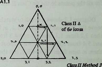
1, Points and 2,1 obtained by trisecting median.
2. Points 1,0 1,1 and 2,0 2,1 obtained from and 2,1
by Equation 1.1.
3. Points 3,1 3,2 obtained by rotating the system
downward.
¶ Appendices
¶ Appendix I: Writing Class II Method 3 Coordinates
I haven’t been able to find an easier method than the following.
Diagram 1.1 shows a 6v example.
-
Divide the vertical median of a Class II triangle face into equal parts for -frequency. This median is:
octahedron: 45°,
icosahedron: , or 31.7174744°,
tetrahedron: , or 54.7356103°.
For the 6v icosa shown, the 3 divisions are bounded at 10.5724915 and 21.1449829. The first of these isn’t a vertex; the second gives us the 6 of 2,1. (Every second division point will fall on a vertex.)
-
Great-circle arcs from these division points meet the triangle’s left and right sides at 90°. To find the of the intersection we use the equation
\tan \Theta_{1}= \tan \Theta/\cos A \label{eq:I.1}Here is 1 /2 the angle at a polyhedron vertex (that is, 45° for the octa, 36° for the icosa, 60° for the tetra). So in the example, the 0 of 1,0 and 1,1 is
\arctan (\tan 10.5724915/\cos 36) = 12.9913757.$$ Similarly, the $\Theta$ of 2,0 and 2,2 is $$\arctan (\tan 21.1449829/\cos 36) = 25.5512604.When we have completed this process we know the of every point down the right and left edges and along the vertical median. And for the icosa the corresponding values are of course 72,0, and 36, respectively.
-
All other points are obtained by rotating the Class II triangle downward the length of one diamond. Thus in the example, if the diamond 0,0-1,0-2,1-1,1 is slid downward its own length till 0,0 falls on the spot vacated by 2,1, then 1,0 will move to 3,1 and 1,1 to 3,2. To accomplish this we use the rotation formulae, Equation 14.1 and Equation 14.2, and the point we move to 0,0 is the one with the same 9 as 2,1, but lying on the 0 meridian 180° away (that is, point 216, 21.1449829). When we do this we find that 1,0 moves to 21.7718193,32.5212749, and 1,1 moves to 50.2281807, 32.5212749. These are 3,1 and 3,2, respectively, which accounts for all the points in the 6v Class II triangle.
Diagram 1.2 shows a detail to watch. In this lOv example, we move the diamond 0,0-1,0-2,1-1,1, as before, and get 3,1 from 1,0, then 3,2 from 1,1, also 4,1 and 4,3 from 2,0 and 2,2, finally 5,1 and 5,4 from 3,0 and 3,3. What about 5,2 and 5,3? We could get them in turn from 3,1 and 3,2, but these points themselves have already been obtained by rotation, and we may have reason to be nervous about accumulating errors, if not here, certainly in some very-high-frequency example in which third- and fourth-generation rotations are conceivable. A better strategy is to move the diamond 0,0-2,0-4,2-2,2, whereupon 1,0 will give us 5,2 and 1,1 will give us 5,3. By suitable choice of a diamond, and faith in symmetry, it is always possible to avoid deriving a point from a point that was itself derived by rotation.
Finally, the reader should notice a quirk in the rotation formulae, of consequence only when, as here, we are relocating points within a system but not moving the whole system. In effect, the two equations answer the question, where does point p,q go when another point m,n is moved to 0,0? A little reflection will convince us that this question has an infinite number of answers, since it specifies only that the distance between two points shall not change. When m,n is at 0,0 then the 9 of p,q will simply be the distance that separates them; in fact Equation 14.1 is nothing but the distance formula (Equation 9.2) with the second-power terms removed. But the 0 of p,q can have any value whatever: p,q can lie anywhere along the lesser circle of center 0,0 and radius 9. It is only when we add a third point, r, s, that the 0 values become meaingful, and then all they specify is that the relationship between the three points shall not have changed; they say nothing about the icosahedron, or whatever it was, from which we took the three points. If all three points have swung, say, 36° westward, their private interrelations are still unvaried which is what the rotation formulae set out to achievethough they have all three come unmoored from the icosa face where we found them. 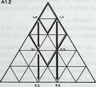
And in fact Equation 14.2 has a habit of swinging things about in this way, seeking as it does a convenient axis of rotation without consulting our preference. But since it rotates everything by the same amount, we have only to find out what it is doing and we shall know what correction to apply. In the example above, sliding the diamond 0,0-1,0-2,1-1,1 straight down the Class II triangle’s median ought to bring 0,0 to 2,1that is, to 36, 21.1449829. In fact 0,0 ends up at 0, 21.1449829, which means that the system swings 36° westward. So we apply a correction of +36° to all values yielded by Equation 14.2.
This fact did not trouble us when we were using the rotation formulae to derive new chord factors for truncation planes, since we always moved both of the points involved and never referred from them to points of the system that had not undergone rotation.
¶ Appendix II: Calculator Routines
Before the introduction of the “scientific” pocket calculator in 1972, spherical coordinates were quite impractical. The basic distance formula (for chord factors) required looking up six different trig functions, manipulating these unwieldy numbers, and taking a square root. Even if a slide rule gave sufficient accuracy (which it doesn’t, except for crude geodesic structures) the need to add or subtract would drive its user to pencil and paper at least three times in the course of computing one chord factor. The calculator gives multiplace accuracy in less than a minute.
Routines for handling our principal equations on the Hewlett-Packard HP-35 are given below. This is a comparatively simple machine with a 4-level stack but only one storage register, and one must sometimes manipulate the stack a good deal to avoid reentering data. The reader may find better procedures of his own. The routines can also be used on other Hewlett-Packard machines such as the HP-21 and HP-45, with the following modifications. (1) Remember to insert shift prefixes where appropriate. (2) Use the alternate routines provided for Equations 13.3,13.4 and 13.7, to accommodate a power function of the form instead of the HP-35’s . (3) On the HP-45 with its addressable storage registers, remember to supply an address for each STO. You may want to rewrite the routines using more than one register and avoiding all data reentry.
The HP-35 routines are read left to right. Each block is either the name of a piece of data or the name of a machine key (t means “enter”). Thus the first seven items in the Equation 9.2 (chord factors of spheres) routine tell you to key the value of 9r, press “enter,” press “cos,” key the value of 02, press “STO,” press “cos,” press “X.”
Chord Factors of Spheres (Equation 9.2)
011 cos 02 STO cos X sin RCL sin X 0i t 02 - 008 X + 2 X
CHS t 2 + V
Chord Factors of Nonspherical Structures (Equation 9.1)
t cos 02 STO cos X xt*y sin RCL sin X 0j t 02 - cos X + 2 X
CHS STO t t RCLX STO R t X r2 t t RCL X STO R t X + RCL
+ V
Radius of an Ellipse (Equation 13.1)
E t X 11 0 STO sin t X X RCL cos t X +
Radius of a Superellipse (Equation 13.3)
- t E xy 111 2.5 t 0 cos STO arc cos sin xy X 2.5 RCLx + *
- l!xx*+y xy
Alternative form, for yx machines:
E t 2.5 y* t t 0 STO sin 2.5 y* X RCL cos 2.5 yx+2.5 1 /x yx
Radius of a Supercircle (Equation 13.4)
- 111 0 STO sin xy RCL cos R Rl Rl R xy + /x x±;yxy
Alternative form, for y* machines:
0 STO sin 2.5 y* RCL cos 2.5 y* + l!x 2.5 l/x yx
Radius When Two System Radii Are Unequal (Equation 13.7)
t 11 0 STO cos RCL sin Ex X Rl R R xy xy + 0 STO sin
Rl Rl R E2 X xy X RCL cos Ex X xy + (x STO 11 Ex
t E2 X xy RCL X
1 /x x*>y xy
Alternative form, for yx machines:
0 STO cos n yX RCL sin Ex X n y* + 0 STO sin E2 X n / X RCL
cos Ex STO X n yx + E2 RCL X n yx x±>y n i/x
Rotation Formulae (Equation 14.1, Equation 14.2)
0 t cos 0x STO cos X x*±y sin RCL sin X 0 t 0x - cos X + arc cos
STO
(Write down value of 02 and continue:)
sin 0 t - sin X RCL sin arc sin
(Value of 02 is now on display.)
Face Angles (Equation 17.4, Equation 17.5, Equation 17.6)
at t CHS X ft STO t X + 11 X R R4- Rl +x+>y + 2 -RCLarc
cos STO
(Write down value of Face Angle and continue:)
sin X + arc sin
(Write down value of Face Angle and continue:)
RCL+ ISOxy-
(Value of Face Angle Cis now on display.)
Dihedral Angles of Spheres (Equation 17.7)
B cos c X STO t XRCLa XSTO - 1 +/ 2 X cXB sin X /xc t X
RCL - X arc cos
¶ Appendix III: HP-65 Programs
Many of the programs that generated data for this book have been filed with the HP-65 Users’ Library. GEODESICS I: Icosa Coordinates (02487A) produces Class I and Class II breakdown data for the #1 triangle and the Class II triangle respectively; the only input needed is the frequency. GEODESICS VII: Icosa Class I Second Triangle (02692) accepts the #1 triangle values as inputs and applies rotation formulae to obtain Triangle #2. GEODESICS VIII: Class IIIcosa Triangles 2, 3, 4, 5 (02701A) accepts data for the Class II triangle (#1 at the top of Diagram 12.5) and generates the coordinates of the other four. GEODESICS VI: Octahedron Coordinates (02691) gives Class I and Class II breakdown values for any frequency. GEODESICS IX: Triacon Coordinates (02734A) applies the methods outlined in Appendix 1 to the icosahedron, octahedron or tetrahedron. A reader who needs data for higher frequencies than the tables in this book offer may find these programs useful; they can either be run on the HP-65 or used as guides to write programs for computers with print-out facilities.
An improved version of Superellipsoid Radii and Chordal Distances (1693A) is reproduced below. It handles ellipsoidal and superellipsoidal structures with one circular cross-section. For structures with neither cross-section circular, GEODESICS III: Superellipsoid Radii (02693A) solves Equation 13.7 to find vertex radii, and GEODESICS II: Chord Factors (02486A) accepts these radii and the vertex coordinates as inputs to give such chord factors as those in Table 15.3.
GEODESICS IV: Face and Dihedral AnglesSpheres (02694A) solves Equations 17.4 through 17.7, using chord factors as inputs. GEODESICS V: Dihedral and Axial Angles: Non-spheres combines Equations 17.8 and 17.9 in a single routine. Its inputs are chord factors, radii (from Geodesics III or from the superellipsoid pro- gram below), and face angles (from Geodesics IV). The results are accurate but the multiple inputs make this method of reaching them relatively cumbersome.
GEODESICS X: Spherical Coordinate Rotation (02700A) handles Equations 14.1 and 14.2, either fortruncations (Chapter 14) or for rotating an entire system (Chapter 15).
Two programs of general usefulness are given below. One computes chord factors for spherical structures between any two points whose 0,0 values are supplied from the tables. It accepts inputs in either decimal degree or arctan notation. The other keeps in storage the expansion and the exponent for an ellipsoidal or superellipsoid al structure with one circular cross-section (see Equation 13.9) and on being given the decimal 0, 0 values of any two points from a table, computes the two radii and the chord factor of the connecting strut. The three columns in the program listings are step number, keystroke, machine code.
SUPERELLIPSOID RADII AND CHORD FACTORS PROGRAM
| RCL 7 | X | ✓ | sin | ||||||||
| RCL 8 | gxiy | RCL5 | X | ||||||||
| g | RCL8 | f-1 | + | ||||||||
| yx | g | ✓ | |||||||||
| RCL2 | yx | + | X | ||||||||
| f | + | f-1 | RCL5 | ||||||||
| TF1 | * | SF1 | X | ||||||||
| CLX | RCL8 | RCL2 | RCL6 | ||||||||
| RCL4 | g | f | X | ||||||||
| /x | cos | ||||||||||
| f1 | g | RCL4 | f | ||||||||
| R-*P | yx | f | / | ||||||||
| g | r | cos | RTN | ||||||||
| ABS | TFl | X | LBL | ||||||||
| EEX | GTO | RCL1 | D | ||||||||
| CHS | B | RCL3 | STO2 | ||||||||
| STO5 | g+ | ||||||||||
| + | f | f | ST01 | ||||||||
| gx L y | SF1 | cos | RTN | ||||||||
| gLSTx | GTO | RCL2 | LBL | ||||||||
| + | A | f | E | ||||||||
| RCL8 | LBL | sin | STO4 | ||||||||
| g | B | X | g+ | ||||||||
| yx | STO6 | RCL4 | STO3 | ||||||||
| g+ | f-! | f | RTN |
Instructions
Store Expansion, , in R7 (key in value and STO 7)
Store Exponent, n, in R8 (key in value and STO 8)
These values need not be stored again for subsequent cases.
Data entry: Key 0, enter, 0, D. (Stores 0 and 0 of first point in R1
and R2.)
Key 0, enter, 0, E. (Stores 0 and 0 of second point in
R3 and R4.)
If a point is reused in a subsequent case its coordinates need not
be stored again.
Run: Press A. After 16 seconds running time, program will halt
and display chord factor. To see radius of first point, press RCL 5.
To see radius of second point press RCL 6.
Comments
Steps 1 to 46 comprise the radius routine, traversed twice. This solves Equation 13.3, using R*-P to obtain sin0 and cos0 in one operation. Steps 15–17 generate a particle of “grit” (0.000000001) which is routinely added to the sine and cosine to ensure against either value ever being zero: this prevents trouble at steps 24 and 30, since zero cannot be raised to a power. For the same reason negative cosines are converted to positive at step 14. The condition of the flag at step 7 determines whether the radius routine operates on point 1 or point 2, and its condition at step 39 determines whether the program will reenter the radius routine or jump to the chord factor routine. Flag is initially unset, set at step 44 prior to second traverse, again unset at step 57 to prepare for new case. Chord factor routine (Equation 9.1) runs from step 47 to step 88.
| LBL | sin | B | tan | ||||||||
| A | X | f1 | STO3 | ||||||||
| RCL2 | RCL4 | tan | RTN | ||||||||
| f | f | ST02 | LBL | ||||||||
| cos | sin | g+ | D | ||||||||
| RCL4 | X | f-1 | STO2 | ||||||||
| f | + | tan | g+ | ||||||||
| cos | STO1 | ST01 | |||||||||
| X | X | RTN | RTN | ||||||||
| RCL1 | CHS | LBL | LBL | ||||||||
| RCL3 | C | E | |||||||||
| + | f1 | ST04 | |||||||||
| f | f | tan | g+ | ||||||||
| cos | ✓ | STO4 | ST03 | ||||||||
| RCL2 | RTN | g+ | RTN | ||||||||
| f | LBL | f-1 |
Instructions
If data are in “arctan” notation:
First point: arctan 0, enter, arctan 0, B (Stored in Rl, R2)
Second point: arctan 0, enter, arctan 0, C (Stored in R3, R4)
If data are in decimal degree notation:
First point: <L , enter, 0, D (Stored in Rl, R2)
Second point: 0, enter, 0, E (Stored in R3, R4)
B and C keys convert arctan to degrees before storage. Program does not tamper with data, and a point that will be reused in a subsequent case need not be reentered.
To obtain chord factor press A. Running time about 4 1/2 seconds.

¶ Index
¶ Bibliography
Khan, Lloyd. 1970. Domebook 1. Vol. 1. Bolinas, CA: Pacific Domes.
———. 1971. Domebook 2. Vol. 2. Bolinas, CA: Pacific Domes.
Lauchner, Julian H., R. Buckminster Fuller, Joseph D. Clinton, Mark B. Mabee, Richard M. Moeller, and Richard Flood. 1968. “Structural Design Concepts for Future Space Missions.” NASA-CR-101577. https://ntrs.nasa.gov/citations/19690020039.
Owen, G. E. 1961. Fundamentals of Scientific Mathematics. Johns Hopkins University Press. https://books.google.com/books?id=L8aEwgEACAAJ.
¶ Source Scans
¶ eBook Formats
In effect demonstrated by Roger S. Tobie, “A Report on an Inquiry into the Existence, Formation and Representation of Tensile Structures” (Master’s thesis, Pratt Institute: 1967). ↩︎
Dowel comes in 3-foot lengths, but tendons are easier to measure in centimeters. ↩︎
This simple approach was pointed out to me by Professor Rufus Isaacs. ↩︎
I am indebted to Roland O. Davis of Goleta, California, for these calculations. ↩︎
These do not run vertex-to-vertex but are by-products of the subdivision system, which at even frequencies cuts triangles in half. ↩︎
See Marks, Fig. 0–4. ↩︎
The class and method terminology is that of Joseph Clinton, “Geodesic Math,” Domebook 2, pp. 106–107. ↩︎
A note in Domebook 2 (p. 112) set out to make this point but had the mis-fortune to get it exactly reversed. The “smoother arcs” and the less equilateral triangles go with Method 2, not Method 1, as investigation of the numbers in the Domebook tables will show. ↩︎
See Martin Gardner’s article in Scientific American (September 1965): 222–234. ↩︎
Derived by Professor George Owen. ↩︎
See Edward Popko, Geodesics (Detroit: University of Detroit Press, 1968), Figs. 15–19; but the geometric proof in his Figure 19 is full of misprints. ↩︎